


 nueva página del texto (beta)
 Inglés (pdf)
 Artículo en XML
 Referencias del artículo
 Enviar artículo por email
 Citado por SciELO
  Similares en
SciELO
Similares en
SciELO 
 Permalink
1. Background
The Mars climate has undergone constant changes in the past. Studying the physical processes involved in such changes is a very challenging task and it will provide a better understanding of the present climate and its future tendency, not only of Mars but also of Earth (Fanale and Jakosky, 1982; McKay, 1999). A physical-mathematical simulation of the climate of Mars could seem less complicated than the simulations of the Earth’s climate, because Mars nowadays lacks oceans, and the small amount of atmospheric water vapor (Spinrad et al. 1963), water ice clouds (Read and Lewis, 2004) and surface frozen water does not allow the existence of a vigorous hydrological cycle. However, simulations of the Martian climate can be complicated by the inclusion of thermodynamic and dynamic processes. One example is the storage of thermal energy in the lower layers of the regolith, which is a thermodynamic process that takes place by the conduction of heat from the surface during the warm season (boreal summer for Northern Hemisphere or boreal winter in the case of the Southern Hemisphere). This energy is returned to the atmosphere during the cold season (boreal winter for Northern Hemisphere or boreal summer in the case of the Southern Hemisphere) by conduction of heat from the lower layers to the surface. During the polar night, this flow of heat to the surface can regulate the growth of the polar ice cap, formed by the condensation of atmospheric CO2. Another example is the development and spread of an incipient dust layer into a major storm. This is a positive radiative-dynamical feedback process, where the vertical velocity of the air increases due to the increase in its heating as a result of the solar radiation absorbed by the extra dust and reemitted (as longwave radiation) to the air. In this process, near the ground, stronger converging winds would be generated, which in turn would increase the dust uplift, reinforcing the storm (Read and Lewis, 2004).
In the present paper we attempt to simulate some aspects of the climate of Mars using an energy balance model of intermediate complexity, the Thermodynamic Climate Model (TCM), already used for the Earth´s climate (Adem, 1982). In the TCM the thermodynamic equation is applied to the atmospheric layer and the surface layer of the regolith together with the thermal conductivity equation. In the atmosphere the meteorological cyclones and anticyclones that transport heat from the equator to the poles, are considered as turbulence and are incorporated in the thermodynamic equation as a horizontal diffusion process using a constant exchange (austausch) coefficient. In this way, dynamic processes are subordinated to the thermodynamic ones. These equations govern the climate state and evolution in terms of atmosphere and regolith temperatures and atmospheric pressure.
The paper is organized in the following manner: first, we present the model’s equations and basic aspects; second, we show the model solutions, followed by results and conclusions.
2. The model
The TCM is a one-layer model (the troposphere) that has been integrated only in the Northern Hemisphere (NH) between ~ 12º and 90º and has been used to simulate past (Adem, 1981a, b; Mendoza et al. 2010), present (Adem, 1982) and future (Mendoza et el., 2016) climate changes of the Earth, as well as for monthly and seasonal forecast of temperature and precipitation (Adem et al., 2000). The first version of the model was global but one-dimensional, with latitude and time as independent variables; this version was used to explain the zonally averaged seasonal temperature in the troposphere, the position and intensity of the tropospheric jet and to formulate a method for seasonal forecast based on the storage of thermal energy in the ocean (Adem, 1963). In the present work, for the first time, we use a global two-dimensional version of the model to simulate the climate of Mars. In the model, the superscripts (*) and (') indicate, respectively, that the variable is a function of height z, or that the variable is a perturbation with respect to a constant reference value (denoted with sub index 0) that is << than such value. In other words, all variables are functions of latitude φ, longitude ψ, height z measured from the surface and time t. The variables of the model (atmospheric temperature, regolith temperature and atmospheric pressure) correspond to mean daily climatic variables. The main forcing of the model is the mean daily insolation, which changes from sol to sol throughout the Martian year. In the present work we will use the term sol, when referring to the Martian day.
Compared to other climate models, the TCM has basically two advantages: (a) physical processes are modeled with intermediate complexity and therefore are easily understandable, and (b) the dynamics is subordinated to thermodynamics, which implies fewer computing resources. So, many simulations can be performed in much less time than for most other climate models that explicitly reproduce dynamics.
2.1 Temperature, pressure, and density
The model considers an atmospheric layer of thickness H with a constant lapse rate Γ. The absolute temperature T* is:
where T (ψ, φ, t) is the temperature at Z = H. We assumed that for z > H the absorption and emission of atmospheric gases is negligible, thus z = H is the radiation boundary of the model. The lapse rate measurements showed temperature profiles that are non-linear functions of the height. Five entry temperature-pressure profiles from Viking Lander 1 (VL1), Viking Lander 2 (VL2), Mars Pathfinder, Spirit and Opportunity are reported by Withers and Smith (2006). For instance, the Spirit profile can be represented by a relatively smooth quadratic curve in a layer between 30 and 80 km, but between 5 and 30 km can be approximated by an isothermal layer. Opportunity showed three thermal inversions between ~ 6 and 80 km, the first one between ~ 8 and 12 km, the second one between ~ 22 and 24 km, and the third one between ~ 56 and 64 km. However, to a first approximation the five profiles can be represented up to ~ 55 km by a lapse rate of Γ = 1.23 K km-1.
The atmospheric pressure p* and density ϱ* are obtained assuming the hydrostatic equilibrium and the ideal gas equations:
where g = 3.72 ms-2 is the gravity acceleration at the surface, R = 192 JKg -1 K -1 is the gas constant (Read and Lewis, 2004), p = (p*)z=H and ϱ = (ϱ*)z=H. We also assume that H is constant, and T (at this level) is variable:
If H s (φ,ψ) is the orographic height relative to the planet´s reference pressure level of ~ 6.4 mb at z = 0 (Smith et al., 1999a), the vertically averaged temperature is:
2.2 The model equations
The temperature T m (φ,ψ,t) is governed by the thermodynamic equation integrated in the atmospheric layer of thickness H - H s . This equation is two-dimensional and has a mathematical structure similar to the one-dimensional equation of the first global version of the TCM (Adem, 1963); that is, it is a linear elliptic differential equation of the second degree, which can be expressed as:
where T m = T m0 + T' m, c 1 = c V ρ m (H - H s ) and c 3 = c 1 /r 0 2; c V = 652.8 Jkg -1 K -1 is the specific heat at constant volume, r 0 = 3389.5 km is the Mars radius (Read and Lewis, 2004) and ρ m is the layer average density given by:
Using (2) and (3) in (7):
where T s is the temperature at z = H s .
In (6) the left-hand side term ST represents the layer’s storage of thermal energy, and the TU term the planetary horizontal turbulent transport of thermal energy, parameterized through an exchange coefficient K. On the right side E T , G 2 and G 5 are, respectively, the fluxes of shortwave and longwave net radiation, the vertical turbulent sensible heat flux from the surface, and the release of latent heat by the CO2 condensation.
We assumed that the upper surface regolith layer has a thickness h r , density ϱ r , specific heat c r and temperature T r . The energy equation of this layer is:
The left-hand side ST r is the thermal energy per unit area column stored in the regolith layer, E r is the shortwave and longwave net radiation, G 1 is the energy gained by the upper regolith layer by heat conduction from the lower layers, and G 3 is the surface thermal energy lost by the vertical turbulent latent heat flux by ice sublimation.
In the diurnal cycle, solar radiation absorbed in the day is stored in the regolith as thermal energy and released at night as heat. Considered a long-time average, we will have a similar process: during the warm Martian season, the solar radiation absorbed by the surface is transmitted by thermal conduction to the lower layers and stored as thermal energy. During the cold season this energy is conducted towards the surface where it is released as heat. In the polar regions this process has an important role in ice sublimation. Then the temperature T r * (at the surface) of each lower layer is ruled by the equation of thermal conductivity:
where k V is the thermal conductivity coefficient, related to the thermal inertia (I T ) which is a function of the layer’s density, specific heat and thermal conductivity (Piqueux and Christensen, 2011):
2.3 Atmospheric radiation
Equation (2) can be expressed as a function of the surface temperature T s and pressure p s at z = H s :
Here (1) is expressed in terms of T s :
The Mars atmosphere is mainly CO2, therefore this gas is the main long-wave absorber of the atmosphere. The partial CO2 density is:
Here M CO2 = 44.01 g/mol, χ CO2 = 0.95, M = 43.34 g/mol (Franz et al., 2017) and r c = M CO2 χCO2/M = 0.96) which are the molecular ideal gas weight, the CO2 molar fraction, the average molecular weight and the mixing ratio, respectively.
Figure 1 shows the partial CO2 density as a function of height obtained from (14) and using (12) and (13) with characteristic surface values T s = 214.6K and p s = 6.4 mb. Using these temperature and pressure values and the lapse rate of 1.23K km-1, the temperature-pressure profile reproduces well the average of the five entry profiles reported by Withers and Smith (2006) mentioned previously.
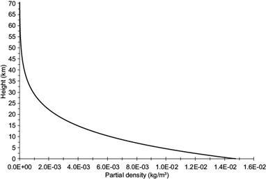
Fig. 1 CO2 partial density of the Martian atmosphere as a function of height, calculated from Eqs. (12), (13) and (14), considering T s = 214.6 K and p s = 6.4 mb.
It is observed that above 55 km the CO2 partial density is negligible. Then we assumed that H = H 0 = 55 km is an appropriate limit for the model upper radiation boundary, and above this level there are no emission gases. The gas mass (kg m-2) in the unit column of height H is:
In (15) we also used (14), the hydrostatic equilibrium equation and considered that p/p s << 1.
The atmospheric emissivity has been found using the E-Trans/HITRAN (E-Trans is a commercial software available at http://www.jcdpublishing.com/about.html) with the HITRAN database version 2004 (Rothman et al., 2005). E-Trans/HITRAN was used successfully for the Earth atmosphere (Mendoza et al., 2017) and now is applied to the Mars atmosphere. When an atmospheric layer is non-isothermal (nor isobaric), E-Trans/HITRAN needs the equivalent temperature and pressure for each component. These variables are defined as the weighted averages with respect to the layer gas content. The CO2 equivalent temperature and pressure are:
In (17) we used (15) and the hydrostatic equilibrium equation, and we assumed that p/p s << 1. Using (14), (15) and (17), U CO2 can be written as:
The lowest equivalent gas pressure that can work with E-Trans/HITRAN is ~ 135 mb (~ 101 Torr). If the surface atmospheric average pressure is ~ 6.4 mb, then according to (17), p e = 3.2 mb. However, we can increase artificially the equivalent gas pressure of the emission layer while keeping constant the gas mass U CO2 , under the hypothesis that its emissivity depends basically on the number of molecules (optical path) in the layer, just as we did previously for the stratospheric layer of O3 on Earth (Mendoza et al., 2017). Then, if U CO2 is constant, (18) implies that:
Here r c = 0.96 and p e = 3.2 mb. Therefore, increasing the pressure to p' e = 135 mb, we found r' c = 0.022. The process of increasing artificially the pressure while decreasing the gas mixing ratio, can overestimate the layer’s emissivity due to the widening. This is caused by the pressure increase and to a lesser degree by the temperature increase of the spectral lines (e.g., Kondratyev, 1969). This will be noted only in the edges of the 15 µm CO2 band (constituted by many superposed lines). In this way, to not overestimate even more the emissivity of this band, we have taken this minimum pressure value (135 mb) with which E-Trans / HITRAN software can work. Figure 2 shows the CO2 atmospheric emission spectrum modulated by the Planck curve at 214.6 K, constructed with the equivalent temperature of 201.9 K, obtained from (16) with T s = 214.6 K, and pressure increased to 135 mb but with the mixing ratio reduced to 22,700 ppm, instead of the typical conditions of 3.2 mb and 960,000 ppm. In Figure 2, the gray area with respect to the total area under the Planck curve is the emissivity, which is equal to 0.24.
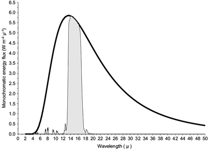
Fig. 2 Monochromatic energy flux (Wm-2 μ-1) from Planck’s spectrum (thick line) and emission bands of the atmospheric CO2 at the Martian surface for 214.6 K (gray area), obtained with E-Trans/HITRAN. We used an equivalent pressure of 135 mb and a mixing ratio of 22 700 ppm. The average width of 15 µm band is ~ 3.5 µ and its area with respect to the total area under the Planck curve is the emissivity ϵ CO2 = 0.24.
Atmospheric emission bands were obtained by the spectrometer IRIS on board of Mariner 9, close to 21º S in a relatively warm region at 280 K (Read and Lewis, 2004). The spectrometer´s average width of the main band of 15 µm is ~ 3.2 µm and the one obtained with E-Trans/HITRAN software is ~ 3.5 µm, which are similar. The emissivity calculated with E-Trans/HITRAN software in order to get a band of 3.2 μm is 0.22, which means that reducing the band width from 3.5 μm to 3.2 μm reduces the CO2 emissivity by 8.5%. Then we can confidently use this spectral calculator for future experiments where the atmospheric mass is increased (for instance for models of the terraformation of Mars).
2.4 Daily insolation at the top of the atmosphere and at the surface
Using the Milankovitch (1920) expression with the orbital Martian parameters:
Here I is the instantaneous solar radiation (insolation) at the surface in the absence of an atmosphere, S 0 = 590 Wm-2 is the total solar irradiance, a 0 is the orbit´s major semiaxis, r is the instantaneous Sun-Mars distance and Z is the zenith angle given by:
where δ is the solar declination angle and ω is the hourly angle ω = 2πt/P, with t the afternoon time and P = 88,750 s the duration of the sol. The angle δ depends on the obliquity η = 25.2º and the areocentric longitude (L s ) expressed in degrees such that ٠º corresponds to the vernal equinox. All the seasons, solstices and equinoxes are named for the NH, so they should be understood as “boreal”. The angles δ, η and L s are related by:
Substituting (21) in (20) and integrating along the sol, we found the average daily insolation (Adem, 1962):
where ω1 is the longitude at noon in radians:
for the polar regions cos ω 1 = -1 and cos ω 1 = 1 at dusk and dawn, respectively, during times longer than one day.
The instantaneous Sun-Mars distance can be found from:
Here e = 0.093 is the orbit’s eccentricity and L s p = 248º is the areocentric longitude at the perihelion (Appelbaum et al., 1993).
Since we are interested in the seasonal climate cycle, we determined the average daily temperatures of the atmosphere (T'm) and of the regolith (T' r ). Then, in E T and E r of (6) and (9), respectively, we must use the average daily insolation given by (23) instead of the instantaneous insolation given by (20). Figure 3 shows the average daily insolation, indicating that during the boreal winter solstice the Southern Hemisphere (SH) gets much more radiation than the NH during the boreal summer solstice, unlike the Earth, where the difference is small. The reason is the Mars eccentricity, which is nowadays 5.6 times larger than that of our planet.
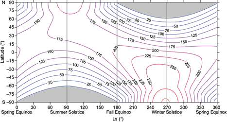
Fig. 3 Average daily solar insolation I d at the top of the Martian atmosphere in Wm-2, as a function of the latitude and areocentric longitude (L s ). The equinoxes (spring and autumn) and the solstices (summer and winter) correspond to L s = 0º, 180º and L s = 90º, 270º, respectively. The red contour corresponds to the largest value.
The atmosphere of Mars is practically transparent to visible radiation (Stephen, 2003), so that the solar radiation extinction through the atmosphere is mainly due to the suspended dust particles and water ice haze (Toigo and Richardson, 2000). The total solar radiation I Tot that reaches the horizontal surface is the sum of the direct plus the diffuse radiations; the I Tot is a fraction of I given by (20), which depends on the zenith angle Z and the optical thickness τ, that we attribute to the atmospheric suspended dust particles. A simplified model to calculate I Tot is taken from Appelbaum et al. (1993):
The Viking missions measured τ in two NH locations, a tropical (22.3º), and a mid-latitude (47.7º) region, finding that during relatively clear atmospheric conditions (spring and summer) τ showed values between 0.2 and 0.7, while during dust storm times (autumn and winter) τ reached values between 1.0 and 3.3 (Appelbaum et al., 1993). However, τ can acquire larger values. During the global dust storm on Mars in June 2018, Opportunity recorded the gradual darkening of the Sun from relatively large and bright to so obscured and small that it could just be perceived; the corresponding values of τ were from 1, for the brightest Sun, to 11, for the almost imperceptible Sun (http://www.nasa.gov/rovers and http://marsrovers.jpl.nasa.gov.).
To model these observations, with the dust storms removed, τ is (Stephen et al., 1999):
The equation for the direct solar radiation (I D ) can be found from the Beer Law, which estimates the light absorption due to dust particles (Appelbaum et al., 1993); it is a function of the optical thickness:
The diffuse solar radiation is just the difference between the I Tot (26) and I D (28).
Equations (26) and (28) are integrated over one sol using the Simpson’s Rule. Figure 4 shows I Tot , for a relatively clear atmosphere (τ = 0.4). Considering average daily values of τ and I Tot , according to the Mars Climate Data Base (MCD) for L s = 200º, 45º N and 120º E, it is found that τ = 0.40 and I Tot = 87.6 Wm-2. According to Figure 4, our result for L s = 200º and 45º N with τ = 0.4 is I Tot 85.0 Wm-2, which suggests some agreement with the MCD.
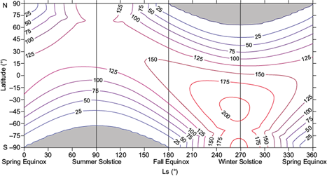
Fig. 4 As in Figure 3, but for the total daily solar radiation (Wm-2) on the horizontal surface, calculated for the conditions of a relatively clear atmosphere with τ = 0.4. The red contour corresponds to the largest value.
2.5 The terms of storage and transport
To estimate the storage term ST, the first left hand side term of (6) (c 1 ∂T' m /∂t), we find that for NH in middle desert latitudes, the factor ∂T' m/∂t is almost of the same magnitude for Mars than for Earth (e.g., in the cold desert of Gobi): 30º and 20º C, respectively, for the winter-summer time span. To calculate the increase of T m from winter to summer on Mars, we use the observed temperature profiles of the Mars Global Surveyor for 6 years (Hinson, 2008), taking temperature at the pressure level p s /2 and at 45 ºN. In the case of Earth, we use the NCEP/NCAR reanalysis data at 500 mb level over the Gobi Desert, for the 30-year period 1961-1990. We use the factor c 1 = c V ρ m (H - H s ) ≈ c V ρ m H = 1.06x10 5 Jm -2 K -1 for the Martian atmosphere, while c V ρ m H = 5.76x10⁶ Jm-2 K -1 for the Earth´s atmosphere, assuming an atmospheric terrestrial layer H ~ 11 km. This implies that the terrestrial ST value is ~ 36 times larger than the Mars value. We have also assumed a thickness of the regolith upper layer of h r = 0.02m, then ρ r = 1.5×10³ kgm -3 and c r = 0.837×10³ J kg -1 K -1 (Fanale and Cannon, 1971), and h r ϱ r c r = 0.8x10⁵ Jm -2 K -1 . For the Earth, the equivalent storage term ST r can be negligible (Adem, 1964). Thus, it is reasonable to assume that for Mars, in (9) the storage term ST r can also be negligible. However, we do not neglect the atmospheric storage term ST for Mars, since it can be important in terraforming experiments, where the mass of the atmosphere is increased due to the greenhouse gases.
Pollack et al. (1990) and Barnes et al. (1993) found that the meridional turbulent heat transport in Mars is important at a global scale. Their calculations showed that such transport around 60 ºN can contribute approximately 5 Wm -2 to the heat balance at those latitudes. On the Earth, meteorological cyclones and anticyclones at mid-latitudes are associated with turbulent horizontal heat transport from the equator to the poles (Adem, 1962). Those terrestrial cyclones and anticyclones obtain almost all of their energy from the baroclinic conversion of the zonal flux, but in Mars this conversion has both a baroclinic and a barotropic character (Holopainen, 1983). In (6), the meridional component of the horizontal turbulent transport (TU), comes from the divergence of the following parameterization:
where v*' ' is the meridional component of the
turbulent or eddy velocity and T*' ' is the
temperature perturbation field; the upper bar means an average over a
sufficiently long time such that
In the terrestrial atmosphere, the parameterization expressed by (29), is
satisfied using an austaush coefficient K ≈ 5×10⁶ m2 s-1 (Stewart, 1945; Adem,
1962). Typical Martian values for the eddy covariance
2.6 Heating functions
The heating functions correspond to the right-hand side terms of (6) and (9). E T and E r can be written as (Adem, 1962):
The energy fluxes E(T*) are the fluxes emitted (or absorbed) by an atmospheric layer at temperature T*; ε is the cloud cover fraction and T c is its temperature; σ = 5.6704×10⁻⁸ Wm-2 K-4 is the Stefan-Boltzmann constant, and α 1 , α 2 and α 3 are the fractional absorptions of insolation (I d ) by the surface of regolith, the gases of the atmosphere (mainly water vapor) and clouds, respectively. In the derivation of (27) and (28), it is assumed that, for long wave radiation, the surface and cloud cover emit as black bodies, but the atmosphere emits only a fraction of the black body emission (Adem, 1962):
where ϵ a is the atmospheric emissivity. For Mars, considering only the CO2 emissivity, ϵ a is equal to the hatched area in Figure 2 divided by the total area under the spectral black body curve. Also, dust, water vapor and ice have important infrared absorptions, with the main dust absorption band 1300-800 cm-1 (7.9 - 12.5 μm) centered at 1075 cm-1 (~ 9 μm) and can contribute with ~ 0.1 to ϵ a in high dust concentration conditions (Ruff and Christensen, 2002). Then in accordance with (27), we express ϵ a as:
The fraction α 1 can be found fromwhere ϵ CO2 is the CO2 atmospheric emissivity. The other right-hand side terms are the dust and water vapor and ice contributions, where we have neglected the overlap of the dust and 15 μm CO2 bands. (Adem, 1964):
where k is a function of the latitude and α is the surface albedo. Adem (1964) also supposes that α2 = a 2 and α 3 = b 3 ε, being a 2 and b 3 functions of the latitude and season.
From (5) and (13) the temperatures T s and T can be expressed in terms of T m , namely:
T s0 and T m0 are found from (1), using T 0 instead of T and taking the reference values z = 0 and z = H/2, such that T s0 = (T*)z=0 = T 0 + ΓH and T m0 = (T*)z=H/2 = T 0 + ΓH/2. For the Earth we have the values of T 0 , Γ and H for a standard atmosphere; with them we find T s0 and T m0 . For Mars we have T s0 = 214.6K, Γ = 1.23 Kkm -1 and H = H 0 = 55km, therefore T 0 = T s0 - ΓH = 147K and T m0 = T s0 - ΓH/2 = 180.8K. Subtracting T s0 , T m0 and T 0 in (35):
For Earth (6) is linear and implicitly integrated over time, and it is convenient for us to assume mathematically that E T and E r are linear functions of T' m and T' r , represented by using Taylor series expansions; then with (36) and assuming that the cloud cover temperature is constant we have for the atmosphere, and from (30):
and for the surface, from (31):
Except for dust, the Martian atmosphere is generally clear, although clouds of both water and CO2 ice can form in certain regions and at certain times of the year. These clouds are not as dense or abundant as those on Earth, but they can reach a significant opacity. Water ice clouds in the equatorial belt are prominent during the aphelion in the boreal summer, and CO2 ice clouds over the polar ice caps in winter (Read and Lewis, 2004). Therefore, clouds albedo would need to be considered and especially its greenhouse effect, because they are thin ice clouds. However, we neglected their radiative effect (shortwave and longwave) in (30), (31), (34), (37) and (38).
The coefficients F n (n = 30….36) in (37) and (38) are:
Here we neglected the orographic effect in F 30 and F 34 because 2 (ΓH s /T0)E(T0) is ~ 8% of E(T 0 ) and 2(ΓH s /T s0 )E(T s0 ) is ~ 6% of E(T s0 ) for a typical value of |H s | = 6 km. The function F(T*) correspond to the atmospheric radiation window (non-hatched area in Figure 2), which is given by:
Assuming that the atmospheric emissivity is roughly independent of temperature:
The turbulent vertical sensible heat flux is:
where c H = 1.2×10⁻³ is the constant heat transfer coefficient, ρ s = p s /RT s is the atmospheric density at the surface, c p = 815 JKg -1 K -1 is the specific heat at constant pressure and |V s | is the surface wind speed with a typical value of 6 ms-1. Using (36) in (41):
where G 0 = c H ρ s c p |V s |(T r0 - T̃s0), and T̃s0 = T s0 + ΓH s /2 ≈ Ts0 because ΓH s /2 is ~ 2% of T s0 for a typical value of |H s | = 6 km.
G 1 is given by:
where T' g = T g - T g0 . We suppose that T g0 is equal to T r0 . T g , which is computed from (10), is the temperature of the layer below the superficial layer.
2.7 Polar thermal energy balance
The main Martian condensation and sublimation processes are those of the CO2 and they are mostly carried out at the poles. Then T' m and T' r will be calculated assuming that in (6) and (9) G 5 and G 3 are zero. At the poles, the CO2 condensation starts at nightfall when the regolith temperature T r descends below the CO2 condensation (or saturation) temperature T sat . The liberated latent heat increases T r up to T sat , which is a function of the atmospheric pressure (Pollack et al., 1981), given by:
where p s is given in hPa.
As the condensation can occur in the atmosphere as well as at the surface, the thermal energy balance is considered in a column including the surface and the atmosphere. Then we must use (6) and (9) together to find the net condensation rate given by G 5 - G 3 . Therefore, considering that in (9) the term ST r has been neglected, then adding (6) and (9), we obtain the rate of change (kg m-2 s-1) of condensed mass m c :
where L is the sublimation latent heat.
Also, to obtain a better result for m c , we will use in (45) the non-linear equations (30) and (31) instead of the linear equations (37) and (38). Then, considering that on the surface ice is in thermal equilibrium with its vapor (CO2 gas) pressure, T r is equal to T sat ; therefore, using (43) with T r = T sat , (45) can be expressed as:
where α p = 1- (α 1 + α 2 + α 3 ) is the planetary albedo, and ST and TU are defined by (6). The first right-hand term is the main contributor to the formation of the ice layer, due to outgoing long-wave radiation from the surface through the window (1 - ϵ a ) in a cloud-free atmosphere, a process similar to the formation of a large scale radiative frost, occurring mainly during the polar night when I d = 0 (this process can be attenuated by the greenhouse effect due to the presence of some CO2 ice clouds over the polar caps during the season cold; see Read and Lewis ENT#091;2004ENT#093;). The second term has a smaller contribution and corresponds to long wave radiation emitted toward space, at the top of the atmosphere (z = H), by atmospheric CO2 and dust. The third term contributes to the ice layer sublimation due to solar radiation after the end of the polar night. The fourth term also contributes to the ice sublimation provided T g > T sat , which happens even during the polar night, and this term modulates the CO2 condensation. The fifth term corresponds to the thermal energy stored in the atmosphere by condensation. And the last term corresponds to the sublimation due to the horizontal turbulent heat transport at mid-latitudes.
In order to calculate T sat , the p s in (44) is determined by using (12) at z =0 , where the pressure is the global mean pressure gM CO2 /A M , where A M is the Martian surface area and M CO2 is the CO2 atmospheric mass, which is equal to the CO2 total available mass (considered constant) minus the condensed mass found from the integral of m c over all the surface area covered by the ice. Then the atmospheric pressure p s at any place on the surface, considering a mostly CO2 atmosphere is:
Equation (47) assumes that even though M CO2 changes day by day, it is rapidly homogenized in all the planet; therefore, the reference pressure (at z=0) is considered uniform throughout. Then (47) shows that the surface pressure depends directly on the CO2 atmospheric mass modulated by the potential relationship of temperatures: ENT#091;T s / (T s + ΓH s )ENT#093;g/RΓ. In (47) the first factor is global and provides the global pressure variation, the second one gives the local thermal-orographic effect, which according to (35) is a function of T m , Γ and mainly H s . The topography H s was obtained from the Mars Orbiter Laser Altimeter (MOLA) on the Mars Global Surveyor (Smith et al., 1999a).
In (46) we calculated (1 - α p ) I d assuming that α 2 and α 3 are negligible, considering only α 1 . Then, neglecting clouds in (34):
where α is determined from https://www.mars.asu.edu/data/irtm_albedo/ and corresponds to the surface Lambertian albedo measured during a time of relatively clear atmosphere by the infrared thermal mapper (IRTM) on the Viking mission (Christensen, 1988). Equation (48) indicates that the planetary albedo, given by α p = 1 - (1 - α) I Tot /I d for I d > 0, is a function of the surface albedo and the atmospheric dust, which reduces the solar radiation from I d to I Tot , increasing the planetary albedo. The atmospheric CO2 that is condensed on the polar surface regions can have a relatively high albedo in visible wavelengths. If the ice is free of dust its albedo will depend on the size of the ice grain varying between ~ 0.8, 0.6 and 0.4 for radii of 0.1, 0.5 and 2.0 mm, respectively. The albedo can be much reduced due to contamination with dust, and then in the model we used an albedo of 0.7 for the seasonal ice in the polar regions (Warren et al., 1990).
2.8 Solution of the model equations
The basic model variables are T' m , T' r and T' g , calculated using the coupled equations (6), (9) and (10). Equations (6) and (9) are integrated implicitly. Following Adem (1965), in (9) the storage term ST r is negligible in comparison with the other terms. Using finite differences in time for the storage atmospheric term ST, if T' mp is the temperature in the previous time step, whose size is ∆t, this term can be expressed as c 1 (T' m - T' mp )/∆t and because the heating functions E T , E r , G 2 and G 1 are linear, (9) becomes a linear and algebraic equation, where T' r is a linear function of T' m and T' g , then substituting T' r in (6), we obtained a differential elliptic linear equation:
where F 1 and F 2 are functions of space and time determined as explained above (see also Adem, 1965). In particular, F 2 depends on the solar radiation fractions absorbed by the surface, atmosphere and clouds, and of the temperature T' g . This temperature in turn is a function of the surface thermal inertia, which is important for the external atmospheric forcing. In fact, the temperature T' m adjusts in such a way that (49) is fulfilled. Equation (49) is solved by finite differences using the Liebmann method, over a grid with a 1º × 1º resolution (the poles are not part of this grid). The boundary conditions are obtained from (49) in each of the two parallels nearest to the poles and are found assuming that the horizontal turbulent transport is zero close to the poles. Then, taking K = 0, the boundary condition is T' m = -F 1 /F 2 . According to Adem (1962), this solution differs significantly from observation in the polar regions of the Earth. However, it allows to determine a boundary condition close to the poles where the solution in spherical coordinates becomes indeterminate. Later we will see that the solution of (49) with this boundary condition is adequate in the polar regions, except in the Southern Hemisphere during autumn and winter. This boundary condition is also used as the first guess in the Liebmann method to determine the final solution for all the other grid points.
In order to solve (49), where ∆t is a sol, we require first to know T' g in (43), which is found by solving (10). Leighton and Murray (1966), using a very simplified thermal model, solved (10) using a resolution of 19 layers: nine equal layers of 1.5 cm and below them 10 equal layers 30 cm thick. Their choice of layers and layer thicknesses has the disadvantage of producing a temperature profile with discontinuity in the spatial derivative between the two layers of different thickness. To integrate (10), we use 24-time steps of 1.025 h to complete one sol. The soil is divided in 40 vertical layers including the surface, which have a variable thickness given by ∆z = h r expENT#091;0.1(k - 1)ENT#093;, with k = 1,2,…,40, in such a way that for the first 20 layers the thickness increases from 0and in the following 20 layers it increases from 0.15 to ~ 1 m, to finish with a total thickness of ~ 10.2 m. The boundary conditions for (10) are (T r *)z1 = T r and (∂T r * / ∂z)z40, here z 1 and z 40 are the first and last middle level layer depths. Knowing T' m from (49) and T' g , considering (9) and that T' r is a linear function of T' m and T' g , then T' r is determined. Having T' m , T' g and T' r , and if the condition T r = T' r + T r0 ≤ T sat is fulfilled, the change rate of condensed mass m c can be found from (46). We have found that the best planetary value for the constants T r0 and T g0 is T r0 = T g0 = 190 K. With such values the linear and nonlinear solutions of (9) coincide. However, the consideration that E T and E r as linear functions (37, 38) of T' m and T' r , implies that during the polar night T r is ~ 6 Cº higher than T sat ; and the condition to apply (46) must change to T r = T' r + T r0 - 6 K ≤ T sat . We ran the model for several years until the seasonal cycles of T m , T r , T g and p s did not change from one year to the next, which occurs between years six and seven. We found that the greater the CO2 total available mass, the more years of running are required to achieve the stability of the seasonal cycle. As a starting point for running the model, we use the representative surface value of -64 ºC for p s = 6.4 mb. This value is just a reasonable guess to reach the Mars climatology.
The adjusted model parameters are the north and south polar thermal inertia and the total available CO2 mass. We performed this adjustment in such a way that the calculated surface atmospheric pressure is as close as possible to the measured pressure by the Viking Lander 1 (VL1) at 22.3º N, 47.9º W and Viking Lander 2 (VL2) at 47.7º N, 225.7º W, and at the same time the calculated maximum condensed mass of south polar ice is closest to that estimated by Hess et al. (1979), (1980), from ~ 7.9 to 8.1×10¹⁵ kg. Examination of the maps of thermal inertia (Mellon et al., 2000) suggested to us a roughly linear trend of thermal inertia with latitude, where we set I T = 270 J m-2 s1/2 K for φ = 89.5º (north polar cap) and I T = 165 J m-2 s1/2 K for φ = -89.5º (south polar cap). These values are within the planetary scale range given by Jakosky (1986): 41.84 to 628 J m-2 s1/2 K. For the total available CO2 mass we found 2.72 × 10¹⁶ kg, while Paige and Wood (1992) and Smith et al. (1999b) found 3.04 ×10¹⁶ kg and ~ 3.2 × 10¹⁶ kg, respectively; Smith et al. (1999b) using this last value found ~ 1.1 × 10¹⁶ Kg for the mass of the south polar cap at L s = 150º.
3. Results
Figure 5 shows, at the beginning of each boreal season (Ls = 0º ENT#091;springENT#093;, Ls = 90º ENT#091;summerENT#093;, Ls = 180º ENT#091;autumnENT#093; and Ls = 270º ENT#091;winterENT#093;), the vertical profile of the regolith temperature computed using (10), corresponding to the VL1 (Fig. 5a) and VL2 (Fig. 5b) sites, and the central part (42.4 ºS, 298.5 ºW) of the Hellas Planitia (HPL) (Fig. 5c). We selected the HPL site because it is in the SH and is the deepest place in Mars (8.2 km below the surface reference level of 6.4 mb). The significant depth of penetration from the surface of the seasonal thermal wave is given by the e-folding length scale (τ 0 k v /ρ r c r π)1/2 (Read and Lewis, 2004); here, τ 0 is the period of the surface thermal signal; then for τ 0 = 5.94 × 10⁷ s (one solar year), the depth for each of the three sites is 0.80, 0.85 and 0.67 m, respectively. In the diurnal cycle (which is not considered in our model), τ 0 = 8.64 × 10⁴ s; then the penetration depth of its thermal wave is ~ 0.03 m, which is not significant for the time scales being examined here. Therefore, the seasonal regulation of the surface regolith temperature is achieved through the thermal conduction from the surface during the warm season, when the thermal wave can penetrate ~ 80 cm, and then this stored energy is returned to the surface during the cold season through the term G 1 in (9). In (45) or (46), G 1 contributes to moderate the CO2 condensation during the polar night. In HPL during its warm season (boreal winter) heat is transmitted from the surface, with a temperature higher than 240 K (Fig. 5c), to the subsurface layers, from where it is transmitted back to the surface during its cold season (boreal summer).
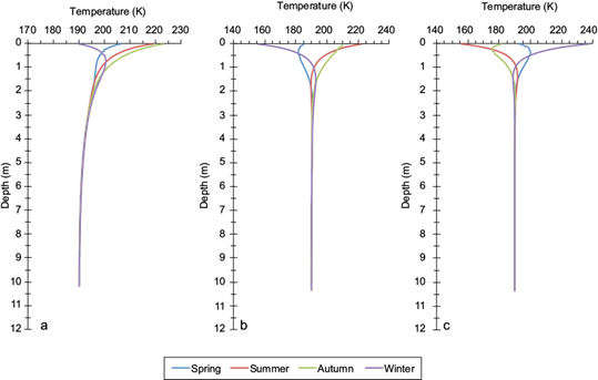
Fig. 5 Vertical temperature profiles of the Martian regolith at the beginning of each boreal season: Ls = 0º (spring), Ls = 90º (summer), Ls = 180º (autumn) and Ls = 270º (winter), at the sites of (a) Viking Lander 1 (VL1), (b) Viking Lander 2 (VL2), and (c) central Hellas Planitia region. The thermal wave is located between the surface and 1 m depth.
The atmospheric temperature at any pressure level is found from (12); in particular at level p s /2, the temperature is:
The temperature (in K) zonally averaged as a function of the latitude appears in Figure 6 for the four yearly seasons. The solid curves correspond to the temperature determined from (50) and the squares are the corresponding seasonal and vertical averages, obtained from the observed temperature profiles by the Mars Global Surveyor during six years (Hinson, 2008). The most important point from this figure is that temperatures between 140 and 160 K are found in the South Pole during spring and summer, and in autumn and winter in the North Pole, which shows some agreement with the observations. The agreement is rough considering that the Hinson (2008) values have low temperature resolution. We would like to point out that, when we used a CO2 emissivity of 0.22 (instead of 0.24), we found an atmospheric average temperature decrease at the p s /2 level of 1.1 K for spring, 1.1 K for summer, 1.2 K for autumn and 1.3 K for winter, supporting our claim that the difference in the band width can be considered negligible as discussed in the last paragraph of subsection 2.3 Atmospheric radiation. In Figure 6, we do not include the temperature curves for the case of the 0.22 emissivity because they are not appreciably different from those of 0.24 emissivity.

Fig. 6 Seasonal atmospheric temperature (K) at the level p s /2 zonally averaged as a function of latitude. The curves are calculated from Eq. (50). The squares are the seasonal and vertical averages over a six-year period from the observed temperature profiles by the Mars Global Surveyor (Hinson, 2008). The seasonal average is calculated along the number of days corresponding to full 90º of L s . To estimate a representative variability of the seasonal averages shown in red squares, we calculate the standard deviation with only the data from the tropical belt (30º N-30º S) because they are the most systematic (observations are scarce at extratropical and high latitudes) and cover practically the surface of half the planet. The average temperature (Tps/2), standard deviation (σ) and number of data (N) in the tropical belt are also shown in this figure.
Figure 7 shows the seasonal variation of atmospheric pressure (in mb) at the surface (z = H s ), as a function of L s , corresponding to the sites of VL1 (Fig. 7a), VL2 (Fig. 7b) and the central part of HPL (Fig. 7c). The solid curves correspond to the calculated pressure using (47), and the dots in Figure 7a and 7b, correspond, respectively, to average daily values observed over a period of four years for the VL1 and three years for the VL2 (Tillman, 1989). In Figure 7c, our estimate in HPL is compared with the daily average values (dotted curve) obtained from the reanalysis results of general circulation models described by Forget et al. (1999) and Millour et al. (2018), which constitute the MCD. Furthermore, from the surface pressure map of Toigo et al. (2013), obtained from CO2 retrievals during the period L s = 0º ‒ 30º, we estimated a surface pressure value for the HPL of ~ 11 mb, that is also in agreement with Figure 7c. The observed seasonal variations of the surface pressure are mainly caused by the CO2 sublimation and condensation processes at the poles. When sublimation of the south polar cap starts (starting at L s =158º and ending around L s = 280º, see Fig. 8), mainly due to solar heating, atmospheric pressure undergoes its maximum increase from ~ 6.8 to ~ 8.9 mb at the VL1 site, and from ~ 7.5 to ~ 9.8 mb at the VL2 site. This corresponds to a CO2 exchange of ~ 8.1 ×10¹⁵ kg from the cap to the atmosphere (Hess et al., 1980). On comparing our calculated pressure change to observation, we notice that for the VL1 the model simulates such change with a phase delay of ~ 12º. For both VL1 and VL2, the observed pressure increases due to sublimation (between L s = 0º and ~ 70º) of the north polar cap are only ~ 0.3 mb, much smaller than for the south polar cap. The calculated increase for both sites is ~ 0.8 mb, larger than the observations. Our results for VL1 and VL2 are comparable to those obtained by Wood and Paige (1992) with an energy balance model; however, in the case of VL1 they get a good agreement with the observations without phase delay. At HPL the first pressure maximum (at L s = 75º) is considerably larger than the second maximum (at L s = 275º). Such difference with respect to the VL1 and VL2 sites is caused by the pressure change, because it is ruled by the CO2 phase changes and by the potential relationship of temperatures (local thermo-orographic effect) shown in Figure 9. In this case, in the first maximum pressure, the factor due to the local orographic effect is 2.15, while in the second maximum this factor is 1.83. In other words, in HPL the local effect strongly modulates the pressure because ΓH s is large and negative (see 47). In this figure, HPL (solid curve), at the SH, the maximum (at L s = 90º) precedes the minimum (at L s = 270º), opposite to VL1 (dot-dashed curve) and VL2 (dashed curve) at the NH.
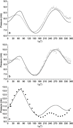
Fig. 7 Pressure (mb) at the surface (z = H s ) as a function of at the sites of Viking Lander 1 (VL1), (b) Viking Lander 2 (VL2), and (c) central Hellas Planitia region. The curves are calculated from Eq. (47), the dots in (a) and squares in (b) correspond to the average daily values observed over a four-year period (VL1) and three-year period (VL2). The dots in (c) are the daily average values obtained from reanalysis of the Mars Data Base and the triangle corresponds to the pressure of ~ 11 mb, estimated from the surface pressure map of Toigo et al. (2013) obtained from CO2 retrievals during the period L s = 0º-30º.
The modeled CO2 mass balance between the atmosphere and the polar caps is shown in Figure 8, presented as in Smith et al. (1999b). The south polar cap (dotted line) starts forming after the spring equinox, reaching its maximum in L s ~ 158º with 8.5 × 10¹⁵ kg, a value slightly greater to that estimated by Hess et al. (1980), 15% lower than that of Smith et al. (1999b) and 43% lower than that of Phillips et al. (2011). This polar cap forms layer by layer from the pole where it is thicker and reduces its thickness as the polar cap extends and reaches latitudes of 40º S, with a superficial density of 100 kg m-2 (Fig.10b); the growth dynamics is ruled by (46). The south polar cap starts decreasing from L s ~ 158º by sublimation and the increase of the daily average solar radiation (Fig. 3). After ~ 230 sols, at L s ~ 300º, the polar cap has completely sublimated, but ~ 46 sols before L s ~ 190º, the north polar cap starts forming (dot-dashed curve), reaching its maximum value of 6.3 × 10¹⁵ kg in ~ 263 sols (at L s ~ 350º) and sublimates completely in 188 sols (at L s ~ 88º). In this way, the planetary surface always keeps a minimum seasonal ice mass (solid curve) of 3.3 × 10¹⁵ kg. The CO2 mass balance implies that the increment (decrement) of the surface total ice mass (solid curve), produces a decrement (increment) of the atmospheric CO2 (dashed curve); then the total available CO2 mass, which is the sum of the condensed and gas masses is a constant (double dot-dashed curve in Fig. 9). The growth of the north polar cap computed with (46) is also by layers (Fig. 10a) starting at the North Pole towards the south; however, this polar cap reaches a smaller extension and has a more circular structure than the south polar cap. The shape and extent of both ice caps simulated by the model, agree well with the shape and extent of seasonal frost on both poles, published by National Geographic (2016).

Fig. 8 Mass balance (1015 kg) as a function of L s of the north polar ice cap (dot/dashed curve), the south polar ice cap (dotted curve) and the total mass of surface ice (solid curve). Also shown are the CO2 atmospheric mass (dashed curve) and the total CO2 available mass (double dotted/dashed curve) considered constant.
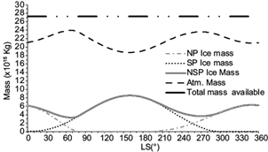
Fig. 9 Temperature ratio ENT#091;T s /(T s - ΓH s )ENT#093;g/RΓ from Eq. (47) as a function of the areocentric longitude (L s ). The curves correspond to: Hellas Planitia region (solid), Viking Lander 1 (dashed) and Viking Lander 2 (dot/dashed).
For polar temperatures about ‒127 ºC, the CO2 ice density is ~ 1.6 × 10³ kg m-3 (Hess et al., 1979), then a superficial layer of 100 kg m-2 is equivalent to a layer of 6.3 cm of thickness. Thereupon, in Figure 10, if curves of equal surface density are multiplied by a factor of 0.063, we find curves of equal ice thickness in centimeters. In this way, the thickness range of the north and south polar caps is between 6.3 to 44.1 cm. Hess et al. (1979) estimated a south polar cap average thickness of 23 cm. Due to Kepler’s Second Law, the south polar night (from L s = 0º to L s = 180°, Figs. 3 and 4) lasts 373 sols, which exceeds in 77 sols the north polar night (from L s = 180º to L s = 360º), which lasts 296 sols. This is one of the main reasons why the ice cap at the South Pole is more extensive and lasts longer than the North Pole cap, although the South Pole is ~ 4 km above the average reference level (~ 6.4 mb), which reduces the condensation temperature. In comparison, the North Pole is ~ 2 km below the reference level, which increases the condensation temperature, enabling the CO2 condensation.
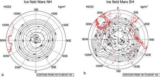
Fig. 10 Ice mass (kg m-2), calculated from Eq. (46), at (a) North Pole for L s = 342º (end of boreal winter) and (b) South Pole for L s = 150º (end of boreal summer). The red contours indicate the reference level z = 0.
As mentioned above, the polar cap starts forming at the beginning of the polar night (hatched area in Fig. 3), reaching its maximum mass at the end of the polar night, resulting in a time delay between the polar mass evolution (Fig. 9, dotted curve for the South Pole and dot-dashed curve for the North) and the insolation (Fig. 3). From the right-hand side of (46), we notice that this maximum occurs when the sum of the third and fourth terms are equal to the sum of the first two terms, then ∂m c / ∂t = 0. The cap’s albedo (third term) and the regolith thermal conductivity (fourth term) produce the delay. That is to say, in relation to the third term, when the polar night ends (I d > 0) the ice begins to reflect radiation, delaying its sublimation, and in relation to the fourth term, when the Sun begins to heat the surface, the lower layers of the regolith maintain a temperature less than the surface temperature (Fig. 5), so that (T g - T sat ) < 0; therefore the fourth term, which is positive, represents a heat flow to the lower layers of the regolith so that it also has the effect of delaying the sublimation of ice.
4. Conclusions
1. Assuming a CO2 atmosphere, we calculate its emission spectrum with E-Trans/HITRAN, resulting in the band of 15 mm (13.5-17 mm) and two large spectral transparent regions on both sides of it, through which the radiation emitted by the regolith and ice caps (considered as black bodies) goes toward space. We also include the atmospheric solar radiation extinction by dust and its longwave emission.
2. The thermodynamic equation establishes the energy balance between the absorbed solar radiation and the outgoing longwave radiation, incorporating also as heating mechanisms the latent heat released by CO2 condensation, the sensible heat flux from the surface to the atmosphere, the latent heat flux due to the CO2 ice sublimation, the heat exchange between the surface regolith layer and its lower layers, and the atmospheric planetary scale horizontal turbulent heat transport with an exchange coefficient of 3.7 × 10⁵ m2 s‒1, which is an order of magnitude smaller than that employed in the terrestrial troposphere.
3. The regolith vertical temperature profile is explicitly determined using thermal inertia. The regolith surface layer temperature results from the balance of the net shortwave and longwave radiation, the thermal conduction from the lower regolith layers and the flux of sensible heat given to the atmosphere. The seasonal regulation of the surface regolith temperature is achieved through the thermal conduction from the surface during the warm season, when the thermal wave can penetrate ~ 80 cm, and then this stored energy is given back to the surface during the cold season. In this process the thermal inertia plays an important role because the e-folding length scale (τ0 k v /ρ r c r π)1/2 = (τ0/π)1/2 IT/ρ r c r is directly proportional to the thermal inertia and inversely proportional to the volumetric specific capacity (ρ r c r ).
4. The Martian polar caps are formed by the atmospheric CO2 condensation during the polar night in a process similar to that of a planetary scale frost, due to the outgoing infrared radiation emitted by the surface (which is assumed to emit as a black body), through the two transparent spectral regions mentioned in (1). Our model can predict the thickness and extent of polar ice caps and consequently the seasonal variation of atmospheric pressure on the surface, which agrees reasonably well at the sites of VL1 and VL2. In the Hellas Planitia case the model has a rough agreement with the MCD.
5. We found explicitly that the seasonal surface pressure variations are modulated by two factors: one associated with the global CO2 mass Mars balance and the other due to the local thermal-orographic effect. The latter is manifested in the seasonal surface pressure cycle in the Hellas Planitia.
6. The thermodynamic model of Mars that we have developed here can be used in the future to simulate some physical processes that we did not consider in this work, such as the possible greenhouse effect of polar clouds, the climatic effect of the albedo of the polar cap modified by dust pollution, and the warming of the Martian atmosphere by the increase of some greenhouse gases such as CO2 itself, which could be used to carry out the terraformation of Mars or the modelling of the solar minima, in order to assess their influence on the Mars climate.

