


 nueva página del texto (beta)
 Inglés (pdf)
 Artículo en XML
 Referencias del artículo
 Enviar artículo por email
 Citado por SciELO
  Similares en
SciELO
Similares en
SciELO 
 Permalink
1. Introduction
Mexico is located within the field of influence of tropical cyclones in its different scales (tropical depressions, tropical storms and hurricanes), that are generated both in the Pacific Ocean and in the Atlantic Ocean (Jáuregui, 1989). The intense rains associated with these phenomena can cause flooding and landslides not only on the coasts but also in the interior of the territory, causing loss of human life and considerable economic damage, which can sometimes have catastrophic tints (Aparicio, 1998; Douben, 2006). The increase in floods has occurred particularly in urban areas, negatively affecting the normal functioning of the social, service, economic and financial sectors, among others, leaving the population with fewer resources and in greater vulnerability (Benjamín, 2008). In addition, Mexico is also frequently affected by other meteorological phenomena, such as cold fronts and mesoscale convective systems (Hernández-Uribe et al., 2017), independently of cyclonic activity.
The state of Puebla has historically presented the problem of flooding. The summary of damages caused by rains, floods, and tropical cyclones for the year 2008 amounted to 2070 people affected, 414 damaged homes and four deteriorated schools, adding economic damages for a total of 2.5 million pesos (SEGOB, 2009).
The Comisión Nacional del Agua (National Water Commission, CONAGUA) informed that rainfall recorded in the northern and northeastern mountains of the state of Puebla for August 10, 2017 as a result of Hurricane Franklin’s passage, broke various historical records. In the Zacapoaxtla weather station, 281 mm of rainfall were recorded, which exceeded the historical maximum of 204 mm recorded on August 9, 2012. Meanwhile, a precipitation of 225 mm was recorded at La Soledad station, a value that exceeds the historical maximum of 212 mm recorded on August 8, 1979. Lastly, the Zaragoza station reported 198 mm of precipitation, higher than the historical maximum of 141.1 mm of August 5, 1975 (CONAGUA, 2017). The Atlas of water vulnerability to climate change in Mexico (Arreguín-Cortés et al., 2015), points out that the municipalities of Cuetzalan del Progreso and Zacapoaxtla, located in the northwest of the state, present a high risk given the current rainfall and tropical cyclone conditions.
In the face of this problem, Numerical Weather Prediction (NWP) constitutes a basic tool to understand, explain and predict the behavior of the atmosphere. The Weather Research and Forecasting (WRF) model has a great acceptance and is used worldwide, both by the scientific community, academics, predictors and decision makers. However, like other dynamic and statistical models, WRF is not perfect, so it is necessary to evaluate its performance in each region. For the particular case of the state of Puebla, the performance of the WRF model for high spatial resolution forecasts of precipitation (which allows the quantitative determination of the degree of confidence and defines the set of optimal physical conditions) has not been evaluated.
The two main objectives of this research were to quantitatively evaluate the performance of the WRF model to simulate precipitation in the state of Puebla, considering different combinations of physical parameters, and compare the results with the rain records obtained from the weather stations during the summer of 2017; and to determine the optimal configurations of the WRF model for obtaining its best performance in the state of Puebla.
2. Dataset and methods
In the particular sense of the experimental approach, one or more independent variables are intentionally manipulated (alleged causes background) to analyze the consequences of this procedure on one or more dependent variables (supposed consequential effects) within a control situation for the researcher (Campbell and Stanley, 2012; Creswell, 2013; White and McBurney, 2013; Babbie, 2014; Hernández-Sampieri et al., 2014).
This study is quantitative and experimental. It considers independent variables (the physical parameterizations of the WRF model) and a dependent variable (the rainfall precipitation generated by the WRF model). The manipulation or variation of independent variables was done in eight degrees. Each one of these levels comprises a group in the experiment, corresponding to the variation of the parameters of microphysics (mp_physics), convection (physics), planetary limit layer (bl_pbl_physics), surface layer (sf_sfclay_physics), soil surface (sf_surface_physics), short wave radiation (ra_lw_phphics), long wave radiation (ra_sw_physics) and the time interval between calls to the convection parameterization (cudt).
There is no rule to determine the number of independent and dependent variables that should be included in an experiment. This depends on the approach to the research problem and the existing limitations (Henríquez-Fierro and Zepeda-González, 2003).
The spectrum of combinations of possible physical parameters in the WRF model is very wide, more than 16 million in the ARW core. For this study, a total of 768 experimental groups were defined, each corresponding to the different levels of variation of the selected physical parameters.
To measure the effect of different experiments, statistical metrics were applied between the simulated precipitation and the accumulated rainfall records in 24 h in weather stations installed in the state of Puebla, where summers are rainier than other seasons of the year. For this reason, summer (from June 1 to August 20, 2017) was chosen as the study period. Further, during this time, the state of Puebla received the onslaught of Hurricane Franklin, which caused torrential rains that exceeded the historical highs in the state.
2.1. Study zone
The state of Puebla is located in the central part of Mexico. It borders to the north with the states of Hidalgo and Veracruz; to the east also with Veracruz and Oaxaca; to the south with the latter and Guerrero, and to the west with this state, Morelos, Mexico, Tlaxcala and Hidalgo (Tamayo, 1996). It has an area of 34 290 km2, which represents 17% of the total national space. It is characterized by a wide topographical heterogeneity because it houses four major biogeographical provinces: The Sierra Madre Oriental, the coastal plain of the North Gulf, the Neovolcanic Axis, and the Sierra Madre del Sur. This geomorphological diversity causes marked changes in altitude, which give rise to a wide variety of climates, dominating the temperate climates that cover most of the territory, followed by warm and semi-arid climates. The climatic heterogeneity is due, in part, to the fact that as altitude increases, temperature decreases and 65% of the territory of Puebla is composed of mountainous topography and hills.
2.2. Description of the WRF model
The performance of numerical models of weather prediction has increased in the last 40 years due mainly to four factors (Kalnay, 2003): (1) The increase in computing power of supercomputers, allowing a finer numerical resolution and fewer approximations in operational atmospheric models; (2) the improvement of the representation of small-scale physical processes within the models (clouds, precipitation, turbulent heat transfer, humidity, momentum and radiation); (3) the use of more accurate data assimilation methods, which results in an improvement of the initial conditions for the model, and (4) the increase in data availability, especially satellite and aircraft data on the oceans and the southern hemisphere.
The main features of the WRF model revolve around its non-hydrostatic dynamics and its ability to process spatial resolutions of a few kilometers (Moya-Álvarez and Ortega-León, 2015). About its structure, the WRF model has two dynamic cores (Advanced Research WRF [ARW] and Nonhydrostatic Mesoscale Mode [NMM]), a data assimilation system, and a software architecture that allows the application of parallel computing to perform simulations (Skamarock et al., 2008). In this study, the dynamic core WRF-ARW version 3.9.1.1 was used. The WRF modeling system requires external data sources and consists of three main modules: (1) the WRF preprocessing system (WPS); (2) the ARW solver, and (3) third-party postprocessing and visualization tools.
2.3. Dataset
The forecast accuracy of the models lies primarily in a good description of the initial state of the atmosphere. This initial state, analysis or first approximation is created by an optimal combination between observed data and a short-term forecast derived from a previous analysis through a process known as data assimilation. According to Zepka (2011), for satisfactory results regarding the predictability of a storm or any adverse weather phenomenon characterized by very small spatial and time dimensions, high-quality input data with high temporal and spatial resolutions are necessary, as well as a high-resolution model.
The WRF model requires knowledge of the initial and boundary conditions for the simulation period at constant time intervals, information which is usually incorporated from global data. For this study, we chose to use the data from the Global Forecast System (GFS) model, which is a reference for operational forecasting and research studies. GFS data was downloaded from ftp://ftp.ncep.noaa.gov/pub/data/nccf/com/gfs/prod.
Daily rainfall records were obtained from the Hydrological Information System (HIS) developed in the Surface Water and River Engineering Management of CONAGUA, through the site http://148.204.8.145. The HIS is a system sponsored by the World Meteorological Organization (WMO) through the Water Management Modernization Program.
Fifty-four weather stations with at least 80% data in the study period were selected as sampling units. Table I lists the 54 selected weather stations with their corresponding keys, and Figure 1 their geographical location within the state of Puebla.
Table I List of the 54 weather stations selected in the state of Puebla.
| No. | Key | Name | Latitude | Longitude | Altitude (masl) |
| 1 | ACHPB | Alchichilca | 19.450000 | -97.418056 | 2340 |
| 2 | ACJPB | Acajete | 19.062500 | -97.934167 | 2330 |
| 3 | ADOPB | Acatlán de Osorio | 18.277222 | -98.055000 | 1270 |
| 4 | AFRPB | Africam | 18.942500 | -98.135833 | 2120 |
| 5 | AHAPB | Ahuatepec | 18.854167 | -97.920833 | 2000 |
| 6 | AHUPB | Ahuazontepec | 20.033056 | -98.148056 | 2216 |
| 7 | APAPB | Apapantilla | 20.406944 | -97.845000 | 2970 |
| 8 | ATXPB | Atlixco | 18.921111 | -98.420833 | 1855 |
| 9 | AVCPB | Ávila Camacho | 20.385833 | -97.881111 | 240 |
| 10 | CDSPB | Cd. Serdán | 18.987222 | -97.441667 | 2550 |
| 11 | CEMPB | Cemex | 18.968889 | -97.958333 | 2225 |
| 12 | CHIPB | Chietla | 18.516111 | -98.579167 | 929 |
| 13 | CHLPB | Cholula | 19.068611 | -98.318056 | 2155 |
| 14 | CHSPB | Chila de la Sal | 18.109722 | -98.567778 | 940 |
| 15 | CNAPB | C.N.A. | 19.022778 | -98.198611 | 2150 |
| 16 | CNGPB | Chignahuapan | 19.743333 | -98.049722 | 2300 |
| 17 | COAPB | Coatzingo | 18.612778 | -98.164722 | 1210 |
| 18 | CPLPB | Capulac | 19.092778 | -98.059444 | 2430 |
| 19 | CTZPB | Cuetzalan | 20.033333 | -97.516667 | 980 |
| 20 | ECHPB | Echeverría | 18.966111 | -98.275556 | 2075 |
| 21 | ELCPB | El Carmen | 20.083333 | -98.116667 | 2160 |
| 22 | HJTPB | Huejotzingo | 19.101111 | -98.456111 | 2260 |
| 23 | HQCPB | Huaquechula | 18.772222 | -98.540278 | 1580 |
| 24 | HUAPB | Huauchinango | 20.176389 | -98.050833 | 1472 |
| 25 | IZMPB | Izúcar de Matamoros | 18.610833 | -98.466389 | 1260 |
| 26 | LIBPB | Libres | 19.457222 | -97.691111 | 2430 |
| 27 | MAYPB | Mayorazgo 21 Pte. | 19.010556 | -98.231111 | 2122 |
| 28 | NNEPB | Nuevo Necaxa | 20.216667 | -98.000556 | 1364 |
| 29 | OYAPB | Oyameles | 19.700000 | -97.533333 | 2850 |
| 30 | PCRPB | Paso Carretas | 18.918056 | -97.251389 | 2600 |
| 31 | PIXPB | Piaxtla | 18.200000 | -98.264722 | 1119 |
| 32 | PTLPB | Patla | 20.233333 | -97.883333 | 525 |
| 33 | PUOPB | Puebla Observatorio | 19.050000 | -98.166667 | 2179 |
| 34 | QUIPB | Quimixtlán | 19.250000 | -97.616667 | 2070 |
| 35 | RNAPB | Rancho Nuevo (Ayotoxco) | 20.116111 | -97.401667 | 366 |
| 36 | SCRPB | San Cristóbal Caleras | 19.113056 | -98.220000 | 2513 |
| 37 | SMCPB | San Miguel Canoa | 18.735000 | -97.910000 | 2583 |
| 38 | SOLPB | La Soledad | 19.960833 | -97.446667 | 1590 |
| 39 | TDRPB | Tepango de Rodríguez | 20.004444 | -97.792500 | 1560 |
| 40 | TECPB | Tecamachalco | 18.878889 | -97.752500 | 2030 |
| 41 | TEHPB | Tehuacán | 18.479167 | -97.395556 | 1648 |
| 42 | TEOPB | Tetela de Ocampo | 19.829444 | -97.805833 | 1725 |
| 43 | TEPPB | Tepexic | 20.000833 | -97.794167 | 1526 |
| 44 | TEZPB | Teziutlán | 19.815278 | -97.956944 | 1950 |
| 45 | TLPPB | Tlacotepec de Díaz | 18.405000 | -96.849722 | 300 |
| 46 | TLXPB | Tlaxco | 20.374167 | -98.040556 | 1065 |
| 47 | TPYPB | Tepeyahualco | 19.489167 | -97.491944 | 2924 |
| 48 | TYAPB | Tepeyac | 18.483611 | -96.861389 | 100 |
| 49 | UDSPB | Universidad de la Sierra | 20.176389 | -98.050833 | 1472 |
| 50 | VENPB | Venustiano Carranza | 20.510278 | -97.675833 | 1200 |
| 51 | XDJPB | Xicotepec de Juárez | 20.277222 | -97.956944 | 1180 |
| 52 | ZCPPB | Zacapoaxtla | 19.859722 | -97.585000 | 2045 |
| 53 | ZOQPB | Zoquitlán | 18.332222 | -97.011389 | 2175 |
| 54 | ZRGPB | Zaragoza | 20.178611 | -97.832778 | 2493 |
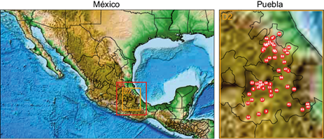
Fig. 1 Geographical location of the selected weather stations in the state of Puebla (right). The station number corresponds to the list of stations in Table I. Experimentation domains with the WRF model (D1 [mother domain, red] and D2 [nested domain, orange]) are marked on the map of Mexico (left).
2.4. Experiment design
Two domains were defined for the execution of the WRF model, the mother domain with a spatial resolution of 16 km and a nested domain with a resolution of 8 km. Only simulated precipitation in the nested domain was used to evaluate the performance of the WRF model in the state of Puebla. Table II shows the fixed parameters selected for experimentation with the WRF model.
Table II Fixed parameters selected for experimentation with the WRF model.
| Parameter | Description | Mother domain | Nested domain |
| dx | Grid length in x direction (m) | 16 000 | 8000 |
| dy | Grid length in y direction (m) | 16 000 | 8000 |
| map_proj | Map projection | Mercator | Mercator |
| time_step | Time step for integration in integer seconds | 96 | 96 |
| history_interval | History output file interval (min) | 180 | 60 |
| ref_lat | Central latitude of the mother domain | 19.3453 | 19.3453 |
| ref_lon | Central length of mother domain | -97.9065 | -97.9065 |
| e_we | End index in x direction (west-east) | 47 | 59 |
| e_sn | End index in y direction (south-north) | 51 | 67 |
| i_parent_start | Starting lower left corner I-indices from the mother domain | 1 | 8 |
| j_parent_start | Starting lower left corner J-indices from the mother domain | 1 | 8 |
As mentioned above, 768 experiments with the WRF model were executed, each one corresponding to one of the possible combinations of the different physical settings selected. Each parameterization was varied in two options, except for the convection parameterization, from which six different ones were selected since precipitation is directly associated with the formation of clouds. However, all the different physical parameterizations affect the simulation of precipitation. The combination was selected on a discretionary basis of the compatibility at the run time between different combinations. Table III lists the physical parameters considered in the 768 experiments.
Table III Physical parameters considered in the 768 experiments.
| Option number | Parameterization |
| Microphysics | |
| 2 | Lin et al. scheme |
| 4 | WRF Single-Moment (WSM) 5-class scheme |
| Convection | |
| 1 | Kain-Fritsch (new Eta) scheme |
| 2 | Betts-Miller-Janjic scheme |
| 3 | Grell-Devenyi ensemble scheme |
| 5 | Grell 3D ensemble scheme |
| 6 | Modifed Tiedtke scheme |
| 14 | New GFS simplified Arakawa-Schubert scheme from YSU |
| Planetary boundary layer | |
| 1 | YSU scheme |
| 2 | Mellor-Yamada-Janjic (Eta) TKE scheme |
| Surface layer | |
| 1 | Monin-Obukhov similarity scheme |
| 2 | Monin-Obukhov (Janjic Eta) similarity scheme |
| Soil surface | |
| 1 | Thermal diffusion scheme |
| 2 | Noah land-surface model |
| Short wave radiation | |
| 1 | RRTM scheme |
| 3 | CAM scheme |
| Long wave radiation | |
| 1 | Dudhia scheme |
| 2 | Goddard shortwave scheme |
| Time step for the convection | |
| 10 | 10 minutes |
| 30 | 30 minutes |
The results of the experiments were sorted by date and weather station, generating a text file consisting of 81 lines which corresponds to the analysis days of the period from June 1 to August 20, 2017. Each line contains 770 columns, the first one containing the date; the second column contains the observed precipitation value, and columns 3 through 770 contain the precipitation value simulated by the WRF model in each of the 768 experiments.
2.5. Metrics to measure the performance of the WRF model
In systems modeling, an essential stage that presents both conceptual and practical difficulties is the validation of the models. An important part of this process is empirical validation, which according to Reynolds (1984) and Mitchell (1997) is done to compare the predictions of the model with observations from the real world. According to Aguilar (1997) and Rauscher et al. (2000), these comparisons should ideally be carried out using appropriate statistical methods, with an acceptable level of confidence, so that the inferences are correct (Barrales et al., 2004).
There are different methods to quantitatively validate numerical forecast models, highlighting the use of simple statistics of bias, root mean square error (RMSE) and Pearson correlation. These parameters were selected because they are not exclusive and can be used together. Among the works that propose and use these statistical parameters for the evaluation of forecast models are Willmott (1982), Pielke (1984), Willmott et al. (1985), Carbonell et al. (2003) and Das et al. (2015).
The selected statistics were applied to each observation site for both the set of observed data (O) and model predictions (P). To the extent that the statistical indicators are favorable and show that the simulated data are approximate to observed data, and that the behavior over time of simulated variables is similar to that observed, it can be concluded that the simulation provides representative data and that the WRF model can simulate the precipitation in the state of Puebla (Gavidia, 2012).
RMSE is a measure of quantitative performance commonly used to evaluate forecasting methods. In this context, RMSE consists in the square root of the sum of the quadratic errors, which captures positive errors as negative; therefore, it expresses both systematic and random errors. RMSE amplifies and penalizes with greater force those errors of greater magnitude (Eq. 1).
where P i is the prediction of the model in position i, O i is the value observed in position i and n is the sample size.
The bias is a consistent, constant, and one-way error. It can be positive (overestimation) or negative (underestimation), which does not depend on the number of elements but on many other factors that can be controlled in general if their existence is suspected and the research is carefully planned and executed (Moya de Madrigal, 2005). This statistic measures the reliability of the model, revealing the systematic error. Not having a bias or having a minimal one is a desirable property which indicates that the forecast is close to reality (Eq. 2).
where P i is the prediction of the model in position i, O i is the value observed in position i, and n is the sample size.
Pearson correlation, denoted by the letter r, is a normalized measure of the linear relationship between two continuous quantitative variables, that is, it measures the dependence of one variable with respect to another independent variable. The Pearson correlation coefficient allows establishing similarities or dissimilarities between variables, to make evident the joint variability and therefore typify what happens with the data (Mondragón-Barrera, 2014 ). The coefficient can score values ranging from -1.0 to 1.0. Values close to 1.0 indicate that there is a strong association between the variables, that is, when one increases the other as well. On the other hand, values close to -1.0 indicate that there is a strong negative association between the variables, implying that when one variable increases, the other decreases. When the value is 0.0, it indicates that there is no correlation, or the correlation is null (Anderson et al., 2008). In the correlation, the dependent variable is not distinguished from the independent one, so the correlation of O with respect to P is the same as the correlation of P with respect to O (Eq. 3).
where O i is the value observed in position i, P i is the prediction of the model in position i, P̅ is the mean observed value, and P̅ is the mean model prediction.
The efficiency multiparameter index (EMI) was used to identify exposed cases with better performance at the state level, which involves four steps:
Calculation of the statistical metrics of bias, RMSE and r in the 768 experimental groups of the 54 observation sites.
Assignment of weights to each experiment according to the level of efficiency in each of the three statistical metrics by location.
Application of the EMI (Eq. 4). EMI values range from 0 to 1, and are interpreted as deficient (0.0 < 0.2), regular (0.2 < 0.4), good (0.4 < 0.6), very good (0.6 < 8.0) and excellent (0.8 ≤ 1.0).
Selection of the experiment with the highest EMI as a reference at the state level.
where EMI e is the efficiency multiparameter index for experiment e, ne the number of experiments, nl the number of locations, nm the number of metrics, and E eml the weight of the experiment e for the metric m and the location l.
3. Results
3.1. Precipitation variability during the study
Given that the year 2017 presented a neutral ENSO condition, rainfall in the state of Puebla during the study period was normal with the exception of August 10, 2017 when in the northern and eastern regions of the state, precipitation from very strong to intense occurred with values exceeding 75 mm accumulated in 24 h. This extraordinary precipitation was caused by hurricane Franklin (category 1), which hit land on August 10 at 00:00 LT in the state of Veracruz and subsequently weakened at 4:00 LT to a tropical storm in the northern highlands of Puebla.
3.2. Analysis and interpretation of results
A first analysis was performed with the results of the statistical evaluation parameters in the 54 locations. Table IV shows the minimum and maximum values in the 768 experiments by weather station and statistical metrics.
Table IV Minimum and maximum values in the 768 experiments by statistical metric and weather station.
| Station key | BIAS | RMSE | r | |||
| Minimun | Maximum | Minimun | Maximum | Minimun | Maximum | |
| ACHPB | 0.01 | 1.16 | 3.18 | 13.52 | 0.07 | 0.85 |
| ACJPB | 0.01 | 1.89 | 5.70 | 34.74 | 0.21 | 0.67 |
| ADOPB | 6.89 | 5.15 | 7.95 | 22.09 | 0.12 | 0.68 |
| AFRPB | 3.77 | 5.26 | 9.85 | 29.51 | 0.06 | 0.52 |
| AHAPB | -0.01 | 3.53 | 6.94 | 28.74 | 0.16 | 0.79 |
| AHUPB | 0.02 | 3.12 | 4.71 | 20.51 | 0.17 | 0.92 |
| APAPB | -0.03 | 9.36 | 15.13 | 30.14 | 0.03 | 0.72 |
| ATXPB | 0.01 | 4.60 | 7.81 | 24.53 | 0.06 | 0.57 |
| AVCPB | 0.01 | 7.04 | 14.46 | 34.25 | 0.01 | 0.50 |
| CDSPB | -0.01 | 1.94 | 4.65 | 19.66 | 0.05 | 0.91 |
| CEMPB | -0.01 | 3.38 | 7.63 | 31.26 | 0.08 | 0.68 |
| CHIPB | -0.01 | 4.57 | 7.82 | 44.97 | -0.02 | 0.49 |
| CHLPB | -0.01 | 7.06 | 9.11 | 27.29 | 0.12 | 0.61 |
| CHSPB | -0.01 | 5.19 | 10.59 | 24.47 | -0.07 | 0.44 |
| CNAPB | 0.01 | 6.17 | 9.46 | 32.02 | 0.04 | 0.51 |
| CNGPB | -0.02 | 1.61 | 5.00 | 26.36 | 0.29 | 0.88 |
| COAPB | 0.01 | 5.64 | 10.86 | 29.90 | 0.00 | 0.87 |
| CPLPB | -0.15 | 2.92 | 6.28 | 31.48 | 0.15 | 0.62 |
| CTZPB | -0.02 | 10.73 | 21.31 | 43.26 | -0.04 | 0.27 |
| ECHPB | -0.01 | 5.73 | 10.91 | 32.81 | 0.09 | 0.63 |
| ELCPB | -0.01 | 3.49 | 5.63 | 32.99 | -0.01 | 0.88 |
| HJTPB | 0.01 | 4.72 | 7.18 | 20.78 | 0.08 | 0.62 |
| HQCPB | 0.03 | 5.50 | 8.28 | 41.70 | 0.09 | 0.68 |
| HUAPB | 0.02 | 6.42 | 9.68 | 32.22 | 0.05 | 0.82 |
| IZMPB | -0.01 | 4.91 | 7.87 | 39.48 | -0.06 | 0.49 |
| LIBPB | 0.01 | 1.70 | 6.15 | 24.74 | 0.04 | 0.78 |
| MAYPB | -0.01 | 4.37 | 9.55 | 33.45 | -0.03 | 0.52 |
| NNEPB | -0.01 | 6.82 | 10.88 | 42.27 | -0.06 | 0.71 |
| OYAPB | 0.03 | 0.50 | 6.69 | 37.95 | -0.06 | 0.98 |
| PCRPB | 0.02 | 3.10 | 7.77 | 35.20 | -0.05 | 0.71 |
| PIXPB | 0.01 | 2.79 | 6.96 | 30.98 | -0.04 | 0.60 |
| PTLPB | -0.01 | 10.22 | 12.84 | 31.63 | 0.07 | 0.68 |
| PUOPB | 0.01 | 5.94 | 10.49 | 33.13 | 0.10 | 0.57 |
| QUIPB | -0.01 | 7.04 | 12.85 | 24.81 | 0.03 | 0.52 |
| RNAPB | 0.01 | 6.92 | 14.66 | 24.42 | 0.04 | 0.74 |
| SCRPB | -0.01 | 7.26 | 11.46 | 31.71 | -0.02 | 0.56 |
| SMCPB | -0.01 | 2.57 | 6.60 | 27.81 | -0.07 | 0.50 |
| SOLPB | -0.01 | 11.99 | 15.53 | 55.27 | -0.07 | 0.86 |
| TDRPB | -0.01 | 12.06 | 16.93 | 39.78 | -0.04 | 0.86 |
| TECPB | -0.01 | 1.09 | 5.58 | 28.05 | -0.06 | 0.93 |
| TEHPB | 0.01 | 0.18 | 4.02 | 18.83 | -0.07 | 0.49 |
| TEOPB | -0.01 | 5.16 | 7.91 | 25.87 | -0.02 | 0.95 |
| TEPPB | 0.01 | 7.63 | 11.64 | 31.04 | 0.02 | 0.73 |
| TEZPB | -0.01 | 5.98 | 25.54 | 33.67 | -0.08 | 0.06 |
| TLPPB | 0.01 | 18.06 | 28.00 | 34.46 | -0.05 | 0.33 |
| TLXPB | 0.02 | 3.20 | 6.92 | 33.49 | 0.03 | 0.51 |
| TPYPB | 0.01 | 1.15 | 3.14 | 15.92 | 0.23 | 0.92 |
| TYAPB | -0.01 | 14.77 | 21.83 | 29.91 | -0.10 | 0.36 |
| UDSPB | 0.01 | 7.23 | 10.58 | 41.61 | 0.05 | 0.77 |
| VENPB | -0.02 | 2.58 | 8.85 | 22.24 | 0.04 | 0.67 |
| XDJPB | 0.01 | 11.48 | 14.69 | 40.96 | 0.06 | 0.78 |
| ZCPPB | -0.01 | 3.73 | 8.25 | 69.73 | -0.06 | 0.98 |
| ZOQPB | -0.01 | 6.47 | 13.73 | 30.46 | -0.04 | 0.27 |
| ZRGPB | 0.01 | 3.54 | 8.75 | 41.73 | -0.07 | 0.98 |
| Mean | 0.19 | 5.49 | 10.13 | 31.85 | 0.03 | 0.67 |
Overall, the 768 experiments tend to underestimate precipitation with negative biases in 33 observation sites, positive biases with a tendency to overestimate precipitation in only six sites, and a mixed trend in 15 locations. Extreme biases in the 54 locations were presented in the interval [-41.96, 18.06].
On the other hand, the different experiments with the WRF model gave RMSEs in the interval [3.14, 69.73]. The lowest RMSE was obtained at ACHPB, AHUPB, CNGPB, CDSPB, TEHPB and TPYPB stations with intervals [3.18, 13.52], [4.71, 20.51], [5.0, 26.36], [4.65, 19.66], [4.02, 18.83], and [3.14, 15.92], respectively. At the opposite end, the WRF model presented the highest RMSE at the HJTPB and TLPPB stations with intervals [15.53, 55.27] and [8.25, 69.73], respectively.
Regarding the Pearson correlation parameter, the results are very varied in the same location. In the 768 experiments both negative and positive correlations were observed, the latter predominating. Under this metric, the WRF model achieved extremely high positive correlations with values greater than 0.9 at the AHUPB, CDSPB, OYAPB, TECPB, TEOPB, TPYPB, ZCPPB, and ZRGPB observation sites. Meanwhile, through the different 768 configurations, the lowest correlations were obtained at stations CTZPB, TEZPB and ZOQPB stations with intervals of [-0.04, 0.27], [-0.08, 0.06] and [-0.04, 0.27], respectively.
A second analysis of results was performed by grouping the observation sites into six groups with ranges of 500 masl, as shown in Table V. It was observed that at altitudes above 2000 masl, corresponding to groups five and six (which together concentrate 50% of the weather stations), the WRF model has better performance, especially in the central and northern region of the state of Puebla, with the exception of the ZOQPB station, where moderate performance was observed. The region in which the WRF model generally presented the lowest performance was the southwest of the state. The contrast between the 768 experimental groups in the same observation site is evident, starting with performances from low to very high. These results emphasize the importance of conducting experiments to determine the appropriate configuration according to the study area. The exception is the CNGPB station, located to the north of the state of Puebla at an altitude of 2300 masl, where the WRF model in all experiments presented medium to very high performance, with bias in the interval [-11.85, 1.61], an RMSE maximum of 26.36 and r greater than 0.29; however, a bad configuration of the WRF model physical parameters in this station would not present, in statistical terms, serious errors in the simulation of precipitation.
Table V Experiments with better performance by statistical metrics and weather station.
| Group number | Station key | Altitude | BIAS | RMSE | r | |||
| Experiment number | Value | Experiment number | Value | Experiment number | Value | |||
| 1 | AVCPB | 240 | 223 | 0.01 | 141 | 14.46 | 141 | 0.50 |
| RNAPB | 360 | 378 | 0.01 | 589 | 14.66 | 269 | 0.74 | |
| TLPPB | 300 | 59 | 6.89 | 538 | 28.00 | 538 | 0.33 | |
| TYAPB | 100 | 60 | 3.77 | 597 | 21.83 | 259 | 0.36 | |
| 2 | CHIPB | 929 | 656 | -0.01 | 314 | 7.82 | 273 | 0.49 |
| CHSPB | 940 | 713 | 0.02 | 390 | 10.59 | 1 | 0.44 | |
| CTZPB | 980 | 55 | -0.03 | 747 | 21.31 | 747 | 0.27 | |
| PTLPB | 525 | 410 | 0.01 | 341 | 12.84 | 341 | 0.68 | |
| 3 | ADOPB | 1270 | 189 | 0.01 | 343 | 7.95 | 343 | 0.68 |
| COAPB | 1210 | 442 | -0.01 | 279 | 10.86 | 279 | 0.87 | |
| HUAPB | 1472 | 242 | -0.01 | 318 | 9.68 | 277 | 0.82 | |
| IZMPB | 1260 | 207 | -0.01 | 718 | 7.87 | 192 | 0.49 | |
| NNEPB | 1364 | 45 | -0.01 | 334 | 10.88 | 140 | 0.71 | |
| PIXPB | 1119 | 133 | -0.01 | 626 | 6.96 | 565 | 0.60 | |
| TLXPB | 1065 | 467 | 0.01 | 725 | 6.92 | 725 | 0.51 | |
| UDSPB | 1472 | 123 | -0.02 | 618 | 10.58 | 9 | 0.77 | |
| VENPB | 1200 | 137 | 0.01 | 621 | 8.85 | 646 | 0.67 | |
| XDJPB | 1180 | 394 | -0.15 | 670 | 14.69 | 670 | 0.78 | |
| 4 | AHAPB | 2000 | 533 | -0.02 | 247 | 6.94 | 372 | 0.79 |
| ATXPB | 1855 | 696 | -0.01 | 222 | 7.81 | 132 | 0.57 | |
| HQCPB | 1580 | 381 | -0.01 | 335 | 8.28 | 6 | 0.68 | |
| SOLPB | 1590 | 226 | 0.01 | 373 | 15.53 | 124 | 0.86 | |
| TDRPB | 1560 | 57 | 0.03 | 493 | 16.93 | 493 | 0.86 | |
| TEHPB | 1648 | 270 | 0.02 | 393 | 4.02 | 397 | 0.49 | |
| TEOPB | 1725 | 153 | -0.01 | 766 | 7.91 | 766 | 0.95 | |
| TEPPB | 1526 | 544 | 0.01 | 10 | 11.64 | 10 | 0.73 | |
| TEZPB | 1950 | 131 | -0.01 | 597 | 25.54 | 456 | 0.06 | |
| 5 | ACHPB | 2340 | 697 | -0.01 | 397 | 3.18 | 512 | 0.85 |
| ACJPB | 2330 | 693 | 0.03 | 398 | 5.70 | 717 | 0.67 | |
| AFRPB | 2120 | 2 | 0.02 | 206 | 9.85 | 206 | 0.52 | |
| AHUPB | 2216 | 235 | 0.01 | 622 | 4.71 | 256 | 0.92 | |
| CEMPB | 2225 | 526 | -0.01 | 739 | 7.63 | 264 | 0.68 | |
| CHLPB | 2155 | 80 | 0.01 | 718 | 9.11 | 707 | 0.61 | |
| CNAPB | 2150 | 157 | -0.01 | 325 | 9.46 | 218 | 0.51 | |
| CNGPB | 2300 | 330 | 0.01 | 638 | 5.00 | 37 | 0.88 | |
| CPLPB | 2430 | 681 | -0.01 | 325 | 6.28 | 135 | 0.62 | |
| ECHPB | 2075 | 534 | -0.01 | 214 | 10.91 | 263 | 0.63 | |
| ELCPB | 2160 | 324 | -0.01 | 323 | 5.63 | 339 | 0.88 | |
| HJTPB | 2260 | 699 | -0.01 | 53 | 7.18 | 452 | 0.62 | |
| LIBPB | 2430 | 541 | -0.01 | 650 | 6.15 | 278 | 0.78 | |
| MAYPB | 2122 | 70 | 0.01 | 213 | 9.55 | 11 | 0.52 | |
| PUOPB | 2179 | 648 | -0.01 | 610 | 10.49 | 610 | 0.57 | |
| QUIPB | 2070 | 559 | 0.01 | 224 | 12.85 | 204 | 0.52 | |
| TECPB | 2030 | 641 | -0.01 | 247 | 5.58 | 248 | 0.93 | |
| ZCPPB | 2045 | 317 | 0.01 | 347 | 8.25 | 752 | 0.98 | |
| ZOQPB | 2175 | 16 | 0.02 | 370 | 13.73 | 328 | 0.27 | |
| ZRGPB | 2493 | 365 | 0.01 | 22 | 8.75 | 394 | 0.98 | |
| 6 | APAPB | 2970 | 220 | -0.01 | 356 | 15.13 | 752 | 0.72 |
| CDSPB | 2550 | 78 | 0.01 | 397 | 4.65 | 636 | 0.91 | |
| OYAPB | 2850 | 269 | -0.02 | 314 | 6.69 | 267 | 0.98 | |
| PCRPB | 2600 | 454 | 0.01 | 586 | 7.77 | 517 | 0.71 | |
| SCRPB | 2513 | 717 | -0.01 | 309 | 11.46 | 21 | 0.56 | |
| SMCPB | 2583 | 210 | -0.01 | 470 | 6.60 | 3 | 0.50 | |
| TPYPB | 2924 | 77 | 0.01 | 127 | 3.14 | 686 | 0.92 | |
| Mean | 0.19 | 10.13 | 0.67 | |||||
3.3. Optimal configuration of the WRF model
Three optimal configurations were determined to execute the WRF model by location, each one corresponding to the experiment which obtained the better performance in the three evaluation metrics. Tables VI, VII and VIII describe the optimal configurations according to the statistical parameters of bias, RMSE, and Pearson correlation, respectively.
Table VI Description of the optimal configuration of the WRF model by location according to the BIAS statistical parameter.
| Station key | Experiment number | Physical parameters | Time step for the convection | ||||||
| Microphysics | Convection | Planetary boundary layer | Surface layer | Land surface | Short wave radiation | Long wave radiation | |||
| ACHPB | 697 | 4 | 6 | 2 | 2 | 2 | 1 | 1 | 10 |
| ACJPB | 693 | 2 | 3 | 2 | 2 | 2 | 3 | 1 | 10 |
| ADOPB | 189 | 2 | 3 | 2 | 2 | 2 | 3 | 1 | 10 |
| AFRPB | 2 | 2 | 1 | 1 | 1 | 1 | 1 | 1 | 30 |
| AHAPB | 533 | 4 | 3 | 1 | 2 | 1 | 3 | 1 | 10 |
| AHUPB | 235 | 2 | 5 | 2 | 1 | 2 | 1 | 2 | 10 |
| APAPB | 220 | 2 | 5 | 1 | 2 | 2 | 1 | 2 | 30 |
| ATXPB | 696 | 4 | 6 | 2 | 2 | 1 | 3 | 2 | 30 |
| AVCPB | 223 | 2 | 5 | 1 | 2 | 2 | 3 | 2 | 10 |
| CDSPB | 78 | 2 | 2 | 1 | 1 | 2 | 3 | 1 | 30 |
| CEMPB | 526 | 4 | 3 | 1 | 1 | 2 | 3 | 1 | 30 |
| CHIPB | 656 | 4 | 6 | 1 | 1 | 2 | 3 | 2 | 30 |
| CHLPB | 80 | 2 | 2 | 1 | 1 | 2 | 3 | 2 | 30 |
| CHSPB | 713 | 4 | 14 | 1 | 1 | 2 | 1 | 1 | 10 |
| CNAPB | 157 | 2 | 3 | 1 | 2 | 2 | 3 | 1 | 10 |
| CNGPB | 330 | 2 | 14 | 1 | 1 | 2 | 1 | 1 | 30 |
| COAPB | 442 | 4 | 1 | 2 | 2 | 2 | 1 | 1 | 30 |
| CPLPB | 681 | 4 | 6 | 2 | 1 | 2 | 1 | 1 | 10 |
| CTZPB | 55 | 2 | 1 | 2 | 2 | 1 | 3 | 2 | 10 |
| ECHPB | 534 | 4 | 3 | 1 | 2 | 1 | 3 | 1 | 30 |
| ELCPB | 324 | 2 | 14 | 1 | 1 | 1 | 1 | 2 | 30 |
| HJTPB | 699 | 4 | 6 | 2 | 2 | 2 | 1 | 2 | 10 |
| HQCPB | 381 | 2 | 14 | 2 | 2 | 2 | 3 | 1 | 10 |
| HUAPB | 242 | 2 | 5 | 2 | 2 | 1 | 1 | 1 | 30 |
| IZMPB | 207 | 2 | 5 | 1 | 1 | 2 | 3 | 2 | 10 |
| LIBPB | 541 | 4 | 3 | 1 | 2 | 2 | 3 | 1 | 10 |
| MAYPB | 70 | 2 | 2 | 1 | 1 | 1 | 3 | 1 | 30 |
| NNEPB | 45 | 2 | 1 | 2 | 1 | 2 | 3 | 1 | 10 |
| OYAPB | 269 | 2 | 6 | 1 | 1 | 2 | 3 | 1 | 10 |
| PCRPB | 454 | 4 | 2 | 1 | 1 | 1 | 3 | 1 | 30 |
| PIXPB | 133 | 2 | 3 | 1 | 1 | 1 | 3 | 1 | 10 |
| PTLPB | 410 | 4 | 1 | 1 | 2 | 2 | 1 | 1 | 30 |
| PUOPB | 648 | 4 | 6 | 1 | 1 | 1 | 3 | 2 | 30 |
| QUIPB | 559 | 4 | 3 | 2 | 1 | 2 | 3 | 2 | 10 |
| RNAPB | 378 | 2 | 14 | 2 | 2 | 2 | 1 | 1 | 30 |
| SCRPB | 717 | 4 | 14 | 1 | 1 | 2 | 3 | 1 | 10 |
| SMCPB | 210 | 2 | 5 | 1 | 2 | 1 | 1 | 1 | 30 |
| SOLPB | 226 | 2 | 5 | 2 | 1 | 1 | 1 | 1 | 30 |
| TDRPB | 57 | 2 | 1 | 2 | 2 | 2 | 1 | 1 | 10 |
| TECPB | 641 | 4 | 6 | 1 | 1 | 1 | 1 | 1 | 10 |
| TEHPB | 270 | 2 | 6 | 1 | 1 | 2 | 3 | 1 | 30 |
| TEOPB | 153 | 2 | 3 | 1 | 2 | 2 | 1 | 1 | 10 |
| TEPPB | 544 | 4 | 3 | 1 | 2 | 2 | 3 | 2 | 30 |
| TEZPB | 131 | 2 | 3 | 1 | 1 | 1 | 1 | 2 | 10 |
| TLPPB | 59 | 2 | 1 | 2 | 2 | 2 | 1 | 2 | 10 |
| TLXPB | 467 | 4 | 2 | 1 | 2 | 1 | 1 | 2 | 10 |
| TPYPB | 77 | 2 | 2 | 1 | 1 | 2 | 3 | 1 | 10 |
| TYAPB | 60 | 2 | 1 | 2 | 2 | 2 | 1 | 2 | 30 |
| UDSPB | 123 | 2 | 2 | 2 | 2 | 2 | 1 | 2 | 10 |
| VENPB | 137 | 2 | 3 | 1 | 1 | 2 | 1 | 1 | 10 |
| XDJPB | 394 | 4 | 1 | 1 | 1 | 2 | 1 | 1 | 30 |
| ZCPPB | 317 | 2 | 6 | 2 | 2 | 2 | 3 | 1 | 10 |
| ZOQPB | 16 | 2 | 1 | 1 | 1 | 2 | 3 | 2 | 30 |
| ZRGPB | 365 | 2 | 14 | 2 | 1 | 2 | 3 | 1 | 10 |
Table VII Description of the optimal configuration of the WRF model by location according to the RMSE statistical parameter.
| Station key | Experiment number | Physical parameters | Time step for the convection | ||||||
| Microphysics | Convection | Planetary boundary layer | Surface layer | Land surface | Short wave radiation | Long wave radiation | |||
| ACHPB | 397 | 4 | 1 | 1 | 1 | 2 | 3 | 1 | 10 |
| ACJPB | 398 | 4 | 1 | 1 | 1 | 2 | 3 | 1 | 30 |
| ADOPB | 343 | 2 | 14 | 1 | 2 | 1 | 3 | 2 | 10 |
| AFRPB | 206 | 2 | 5 | 1 | 1 | 2 | 3 | 1 | 30 |
| AHAPB | 247 | 2 | 5 | 2 | 2 | 1 | 3 | 2 | 10 |
| AHUPB | 622 | 4 | 5 | 2 | 1 | 2 | 3 | 1 | 30 |
| APAPB | 356 | 2 | 14 | 2 | 1 | 1 | 1 | 2 | 30 |
| ATXPB | 222 | 2 | 5 | 1 | 2 | 2 | 3 | 1 | 30 |
| AVCPB | 141 | 2 | 3 | 1 | 1 | 2 | 3 | 1 | 10 |
| CDSPB | 397 | 4 | 1 | 1 | 1 | 2 | 3 | 1 | 10 |
| CEMPB | 739 | 4 | 14 | 2 | 1 | 1 | 1 | 2 | 10 |
| CHIPB | 314 | 2 | 6 | 2 | 2 | 2 | 1 | 1 | 30 |
| CHLPB | 718 | 4 | 14 | 1 | 1 | 2 | 3 | 1 | 30 |
| CHSPB | 390 | 4 | 1 | 1 | 1 | 1 | 3 | 1 | 30 |
| CNAPB | 325 | 2 | 14 | 1 | 1 | 1 | 3 | 1 | 10 |
| CNGPB | 638 | 4 | 5 | 2 | 2 | 2 | 3 | 1 | 30 |
| COAPB | 279 | 2 | 6 | 1 | 2 | 1 | 3 | 2 | 10 |
| CPLPB | 325 | 2 | 14 | 1 | 1 | 1 | 3 | 1 | 10 |
| CTZPB | 747 | 4 | 14 | 2 | 1 | 2 | 1 | 2 | 10 |
| ECHPB | 214 | 2 | 5 | 1 | 2 | 1 | 3 | 1 | 30 |
| ELCPB | 323 | 2 | 14 | 1 | 1 | 1 | 1 | 2 | 10 |
| HJTPB | 53 | 2 | 1 | 2 | 2 | 1 | 3 | 1 | 10 |
| HQCPB | 335 | 2 | 14 | 1 | 1 | 2 | 3 | 2 | 10 |
| HUAPB | 318 | 2 | 6 | 2 | 2 | 2 | 3 | 1 | 30 |
| IZMPB | 718 | 4 | 14 | 1 | 1 | 2 | 3 | 1 | 30 |
| LIBPB | 650 | 4 | 6 | 1 | 1 | 2 | 1 | 1 | 30 |
| MAYPB | 213 | 2 | 5 | 1 | 2 | 1 | 3 | 1 | 10 |
| NNEPB | 334 | 2 | 14 | 1 | 1 | 2 | 3 | 1 | 30 |
| OYAPB | 314 | 2 | 6 | 2 | 2 | 2 | 1 | 1 | 30 |
| PCRPB | 586 | 4 | 5 | 1 | 1 | 2 | 1 | 1 | 30 |
| PIXPB | 626 | 4 | 5 | 2 | 2 | 1 | 1 | 1 | 30 |
| PTLPB | 341 | 2 | 14 | 1 | 2 | 1 | 3 | 1 | 10 |
| PUOPB | 610 | 4 | 5 | 2 | 1 | 1 | 1 | 1 | 30 |
| QUIPB | 224 | 2 | 5 | 1 | 2 | 2 | 3 | 2 | 30 |
| RNAPB | 589 | 4 | 5 | 1 | 1 | 2 | 3 | 1 | 10 |
| SCRPB | 309 | 2 | 6 | 2 | 2 | 1 | 3 | 1 | 10 |
| SMCPB | 470 | 4 | 2 | 1 | 2 | 1 | 3 | 1 | 30 |
| SOLPB | 373 | 2 | 14 | 2 | 2 | 1 | 3 | 1 | 10 |
| TDRPB | 493 | 4 | 2 | 2 | 1 | 2 | 3 | 1 | 10 |
| TECPB | 247 | 2 | 5 | 2 | 2 | 1 | 3 | 2 | 10 |
| TEHPB | 393 | 4 | 1 | 1 | 1 | 2 | 1 | 1 | 10 |
| TEOPB | 766 | 4 | 14 | 2 | 2 | 2 | 3 | 1 | 30 |
| TEPPB | 10 | 2 | 1 | 1 | 1 | 2 | 1 | 1 | 30 |
| TEZPB | 597 | 4 | 5 | 1 | 2 | 1 | 3 | 1 | 10 |
| TLPPB | 538 | 4 | 3 | 1 | 2 | 2 | 1 | 1 | 30 |
| TLXPB | 725 | 4 | 14 | 1 | 2 | 1 | 3 | 1 | 10 |
| TPYPB | 127 | 2 | 2 | 2 | 2 | 2 | 3 | 2 | 10 |
| TYAPB | 597 | 4 | 5 | 1 | 2 | 1 | 3 | 1 | 10 |
| UDSPB | 618 | 4 | 5 | 2 | 1 | 2 | 1 | 1 | 30 |
| VENPB | 621 | 4 | 5 | 2 | 1 | 2 | 1 | 2 | 30 |
| XDJPB | 670 | 4 | 6 | 1 | 2 | 2 | 3 | 1 | 30 |
| ZCPPB | 347 | 2 | 14 | 1 | 2 | 2 | 1 | 2 | 10 |
| ZOQPB | 370 | 2 | 14 | 2 | 2 | 1 | 1 | 1 | 30 |
| ZRGPB | 22 | 2 | 1 | 1 | 2 | 1 | 3 | 1 | 30 |
Table VIII Description of the optimal configuration of the WRF model by location according to the Pearson correlation statistical parameter.
| Station key | Experiment number | Physical parameters | Time step for the convection | ||||||
| Microphysics | Convection | Planetary boundary layer | Surface layer | Land surface | Short wave radiation | Long wave radiation | |||
| ACHPB | 512 | 4 | 2 | 2 | 2 | 2 | 3 | 2 | 30 |
| ACJPB | 717 | 4 | 14 | 1 | 1 | 2 | 3 | 1 | 10 |
| ADOPB | 343 | 2 | 14 | 1 | 2 | 1 | 3 | 2 | 10 |
| AFRPB | 206 | 2 | 5 | 1 | 1 | 2 | 3 | 1 | 30 |
| AHAPB | 372 | 2 | 14 | 2 | 2 | 1 | 1 | 2 | 30 |
| AHUPB | 256 | 2 | 5 | 2 | 2 | 2 | 3 | 2 | 30 |
| APAPB | 752 | 4 | 14 | 2 | 1 | 2 | 3 | 2 | 30 |
| ATXPB | 132 | 2 | 3 | 1 | 1 | 1 | 1 | 2 | 30 |
| AVCPB | 141 | 2 | 3 | 1 | 1 | 2 | 3 | 1 | 10 |
| CDSPB | 636 | 4 | 5 | 2 | 2 | 2 | 1 | 2 | 30 |
| CEMPB | 264 | 2 | 6 | 1 | 1 | 1 | 3 | 2 | 30 |
| CHIPB | 273 | 2 | 6 | 1 | 2 | 1 | 1 | 1 | 10 |
| CHLPB | 707 | 4 | 14 | 1 | 1 | 1 | 1 | 2 | 10 |
| CHSPB | 1 | 2 | 1 | 1 | 1 | 1 | 1 | 1 | 10 |
| CNAPB | 218 | 2 | 5 | 1 | 2 | 2 | 1 | 1 | 30 |
| CNGPB | 37 | 2 | 1 | 2 | 1 | 1 | 3 | 1 | 10 |
| COAPB | 279 | 2 | 6 | 1 | 2 | 1 | 3 | 2 | 10 |
| CPLPB | 135 | 2 | 3 | 1 | 1 | 1 | 3 | 2 | 10 |
| CTZPB | 747 | 4 | 14 | 2 | 1 | 2 | 1 | 2 | 10 |
| ECHPB | 263 | 2 | 6 | 1 | 1 | 1 | 3 | 2 | 10 |
| ELCPB | 339 | 2 | 14 | 1 | 2 | 1 | 1 | 2 | 10 |
| HJTPB | 452 | 4 | 2 | 1 | 1 | 1 | 1 | 2 | 30 |
| HQCPB | 6 | 2 | 1 | 1 | 1 | 1 | 3 | 1 | 30 |
| HUAPB | 277 | 2 | 6 | 1 | 2 | 1 | 3 | 1 | 10 |
| IZMPB | 192 | 2 | 3 | 2 | 2 | 2 | 3 | 2 | 30 |
| LIBPB | 278 | 2 | 6 | 1 | 2 | 1 | 3 | 1 | 30 |
| MAYPB | 11 | 2 | 1 | 1 | 1 | 2 | 1 | 2 | 10 |
| NNEPB | 140 | 2 | 3 | 1 | 1 | 2 | 1 | 2 | 30 |
| OYAPB | 267 | 2 | 6 | 1 | 1 | 2 | 1 | 2 | 10 |
| PCRPB | 517 | 4 | 3 | 1 | 1 | 1 | 3 | 1 | 10 |
| PIXPB | 565 | 4 | 3 | 2 | 2 | 1 | 3 | 1 | 10 |
| PTLPB | 341 | 2 | 14 | 1 | 2 | 1 | 3 | 1 | 10 |
| PUOPB | 610 | 4 | 5 | 2 | 1 | 1 | 1 | 1 | 30 |
| QUIPB | 204 | 2 | 5 | 1 | 1 | 2 | 1 | 2 | 30 |
| RNAPB | 269 | 2 | 6 | 1 | 1 | 2 | 3 | 1 | 10 |
| SCRPB | 21 | 2 | 1 | 1 | 2 | 1 | 3 | 1 | 10 |
| SMCPB | 3 | 2 | 1 | 1 | 1 | 1 | 1 | 2 | 10 |
| SOLPB | 124 | 2 | 2 | 2 | 2 | 2 | 1 | 2 | 30 |
| TDRPB | 493 | 4 | 2 | 2 | 1 | 2 | 3 | 1 | 10 |
| TECPB | 248 | 2 | 5 | 2 | 2 | 1 | 3 | 2 | 30 |
| TEHPB | 397 | 4 | 1 | 1 | 1 | 2 | 3 | 1 | 10 |
| TEOPB | 766 | 4 | 14 | 2 | 2 | 2 | 3 | 1 | 30 |
| TEPPB | 10 | 2 | 1 | 1 | 1 | 2 | 1 | 1 | 30 |
| TEZPB | 456 | 4 | 2 | 1 | 1 | 1 | 3 | 2 | 30 |
| TLPPB | 538 | 4 | 3 | 1 | 2 | 2 | 1 | 1 | 30 |
| TLXPB | 725 | 4 | 14 | 1 | 2 | 1 | 3 | 1 | 10 |
| TPYPB | 686 | 4 | 6 | 2 | 1 | 2 | 3 | 1 | 30 |
| TYAPB | 259 | 2 | 6 | 1 | 1 | 1 | 1 | 2 | 10 |
| UDSPB | 9 | 2 | 1 | 1 | 1 | 2 | 1 | 1 | 10 |
| VENPB | 646 | 4 | 6 | 1 | 1 | 1 | 3 | 1 | 30 |
| XDJPB | 670 | 4 | 6 | 1 | 2 | 2 | 3 | 1 | 30 |
| ZCPPB | 752 | 4 | 14 | 2 | 1 | 2 | 3 | 2 | 30 |
| ZOQPB | 328 | 2 | 14 | 1 | 1 | 1 | 3 | 2 | 30 |
| ZRGPB | 394 | 4 | 1 | 1 | 1 | 2 | 1 | 1 | 30 |
The results show that no single experiment has the best performance for the WRF model in all the observation sites, nor in the three statistical metrics. Although some experiments with high performance in different metrics and observation sites were identified, they were scarce.
The experiment with control number 571 obtained the best performance at the state level according to the EMI, with a very good value of 0.76. Table IX shows the 10 experiments with highest EMI values. After analyzing the 10 best configurations according to the EMI (Table X), it was identified that the settings of the microphysics WRF Single-Moment (WSM) 5-class scheme (option 4), the convection parameterization Grell-Devenyi ensemble scheme (option 3), the planetary boundary layer parameterization Mellor-Yamada-Janjic (Eta) TKE scheme (option 2), and the long wave radiation Goddard Shortwave Scheme (option 2) are kept constant to achieve a comparable performance at the state level.
Table IX Statistical parameters of the 10 experiments with the best EMI at the state level.
| Experiment number | EMI | BIAS | RMSE | r | ||||||
| Minimum | Maximum | Average | Minimum | Maximum | Average | Minimum | Maximum | Average | ||
| 571 | 0.76 | -0.62 | 10.59 | 9.27 | 9.74 | 42.32 | 24.98 | 0.06 | 0.77 | 0.35 |
| 555 | 0.75 | -0.23 | 10.13 | 8.46 | 9.24 | 48.36 | 24.24 | 0.05 | 0.82 | 0.34 |
| 547 | 0.74 | 0.27 | 10.49 | 8.92 | 9.19 | 48.68 | 24.50 | 0.07 | 0.75 | 0.35 |
| 548 | 0.74 | -0.36 | 10.70 | 9.13 | 11.22 | 46.69 | 24.83 | 0.06 | 0.79 | 0.36 |
| 572 | 0.73 | -0.05 | 9.69 | 9.00 | 10.50 | 39.68 | 24.05 | 0.06 | 0.83 | 0.36 |
| 551 | 0.72 | -0.23 | 11.86 | 6.66 | 9.20 | 39.10 | 22.39 | 0.07 | 0.72 | 0.37 |
| 556 | 0.72 | 0.11 | 8.44 | 8.63 | 10.05 | 42.50 | 23.81 | 0.04 | 0.86 | 0.36 |
| 563 | 0.71 | -0.29 | 13.73 | 6.80 | 7.66 | 37.99 | 22.43 | 0.05 | 0.82 | 0.38 |
| 564 | 0.71 | -0.26 | 13.50 | 6.74 | 7.71 | 32.46 | 21.80 | 0.04 | 0.81 | 0.37 |
| 552 | 0.70 | 0.97 | 11.33 | 6.83 | 10.92 | 37.73 | 21.86 | 0.08 | 0.82 | 0.39 |
Note: experiments were ordered from highest to lowest EMI.
Table X Parameter configuration of the cases exposed with better EMI at the state level.
| Experiment number | Physical parameters | Time step for the convection | ||||||
| Microphysics | Convection | Planetary boundary layer | Surface layer | Land surface | Short wave radiation | Long wave radiation | ||
| 547 | 4 | 3 | 2 | 1 | 1 | 1 | 2 | 10 |
| 548 | 4 | 3 | 2 | 1 | 1 | 1 | 2 | 30 |
| 551 | 4 | 3 | 2 | 1 | 1 | 3 | 2 | 10 |
| 552 | 4 | 3 | 2 | 1 | 1 | 3 | 2 | 30 |
| 555 | 4 | 3 | 2 | 1 | 2 | 1 | 2 | 10 |
| 556 | 4 | 3 | 2 | 1 | 2 | 1 | 2 | 30 |
| 563 | 4 | 3 | 2 | 2 | 1 | 1 | 2 | 10 |
| 564 | 4 | 3 | 2 | 2 | 1 | 1 | 2 | 30 |
| 571 | 4 | 3 | 2 | 2 | 2 | 1 | 2 | 10 |
| 572 | 4 | 3 | 2 | 2 | 2 | 1 | 2 | 30 |
Note: The experiments correspond to those in Table IX but sorted ascendingly by experiment number for clarity.
Figures 2 3, 4, 5, 6, 7 and 8 present the time series corresponding to observed precipitation in comparison to simulated precipitation by the WRF model, which were analyzed in four experiments corresponding to the following parameters: (1) less BIAS, (2) lower RMSE, (3) greater Pearson correlation, and (4) higher statewide EMI. The following four observations were derived from this time series analysis:
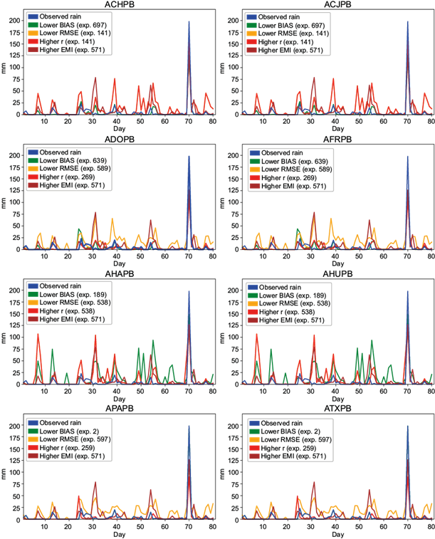
Fig. 2 Time series for the ACHPB, ACJPB, ADOPB, AFRPB, AHAPB, AHUPB, APAPB, and ATXPB stations, showing the comparison between observed precipitation and precipitation simulated by the WRF model in the four experiments with better performance in each locality.
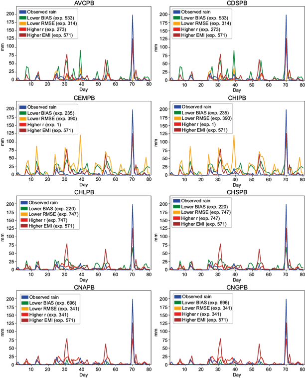
Fig. 3 Time series for the AVCPB, CDSPB, CEMPB, CHIPPB, CHLPB, CHSPB, CNAPB, and CNGPB stations, showing the comparison between observed precipitation and precipitation simulated by the WRF model in the four experiments with better performance in each locality.
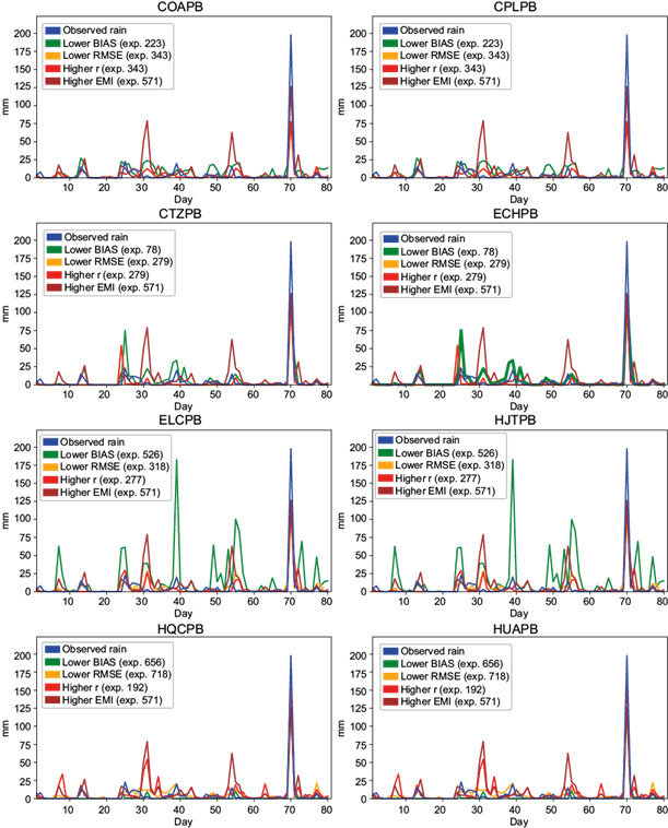
Fig. 4 Time series for the COAPB, CPLPB, CTZPB, ECHPB, ELCPB, HJTPB, HQCPB, and HUAPB stations, showing the comparison between observed precipitation and precipitation simulated by the WRF model in the four experiments with better performance in each locality.
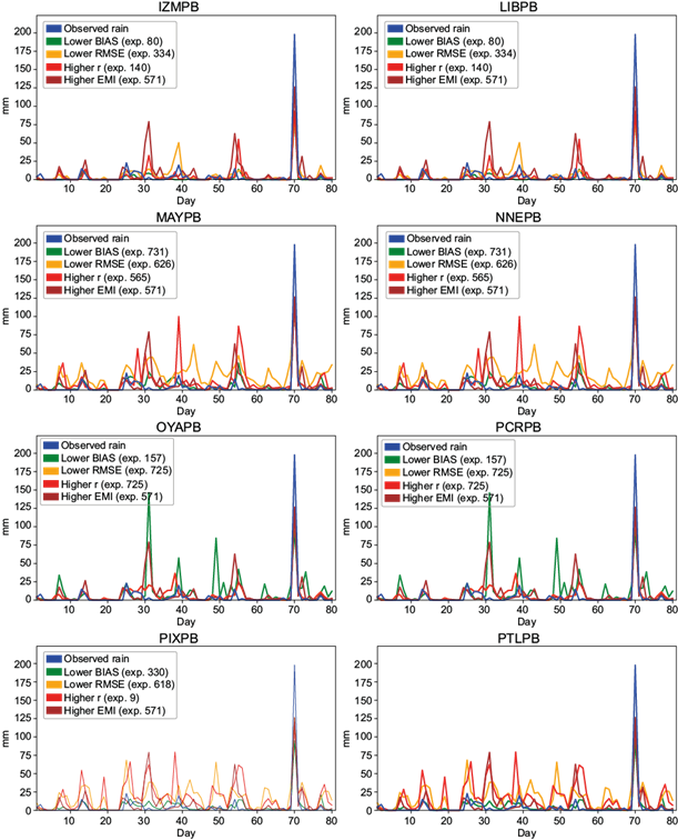
Fig. 5 Time series for the IZMPB, LIBPB, MAYPB, NNEPB, OYAPB, PCRPB, PIXPB, and PTLPB stations, showing the comparison between observed precipitation and precipitation simulated by the WRF model in the four experiments with better performance in each locality.
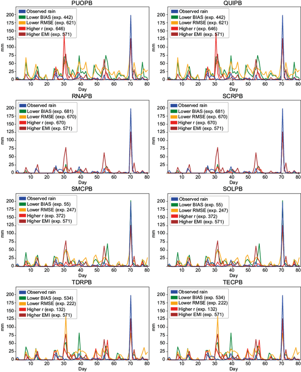
Fig. 6 Time series for the PUOPB, QUIPB, RNAPB, SCRPB, SMCPB, SOLPB, TDRPB, and TECPB stations, showing the comparison between observed precipitation and precipitation simulated by the WRF model in the four experiments with better performance in each locality.
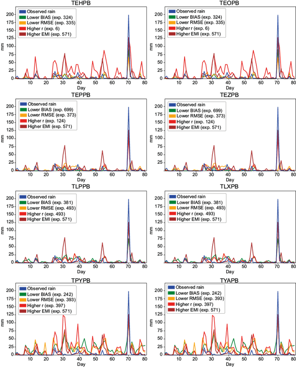
Fig. 7 Time series for the TEHPB, TEOPB, TEPPB, TEZPB, TLPPB, TLXPB, TPYPB, and TYAPB stations, showing the comparison between observed precipitation and precipitation simulated by the WRF model in the four experiments with better performance in each locality.
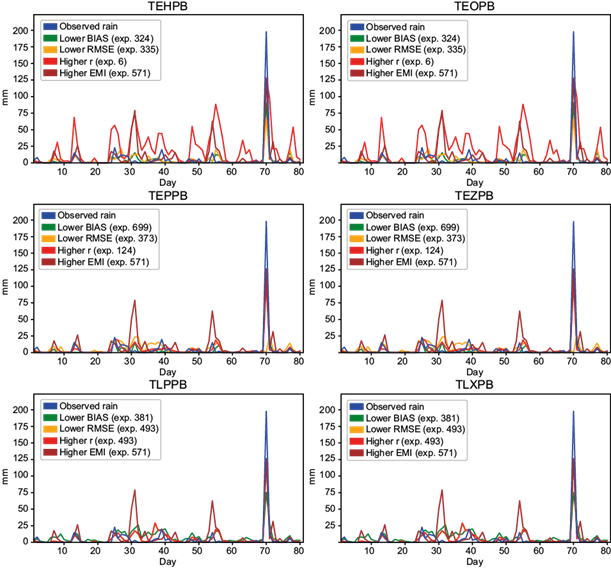
Fig. 8 Time series for the UDSPB, VENPB, XDJPB, ZCPPB, ZOQPB, and ZRGPB stations, showing the comparison between observed precipitation and precipitation simulated by the WRF model in the four experiments with better performance in each locality.
During the study period, the state of Puebla presented a strong rainfall concentration (greater than 25 mm per day) from June 20 to July 10. Intense to extraordinary rainfall (greater than 75 mm per day) also took place at 23 observation sites in the northern part of the state due to Hurricane Franklin on August 10, exceeding the highest historical rainfall at SOLPB, ZCPPB, and ZRGPB stations with records of 225, 281 and 198 mm, respectively.
It was observed that in the CTZPB station, the observed data of extraordinary rainfall occurred on August 10 show a two-days forward displacement, while at the TEZPB station data show a one-day backward change . Therefore, there might be an error in the capture dates at these two observation sites, which would explain the poor performance of the WRF model at these locations.
Although the three best experiments identified by location (corresponding to the lower bias and RMSE, and the higher Pearson correlation) show an outstanding performance of the WRF model in the precipitation simulation, they do not display the same performance in a homogeneous way in the 54 observation sites.
The performance of experiment 571, with the highest EMI at the state level in the 54 observation sites, is comparable to that obtained in the experiments that presented better performance locally for the bias, RMSE and r parameters.
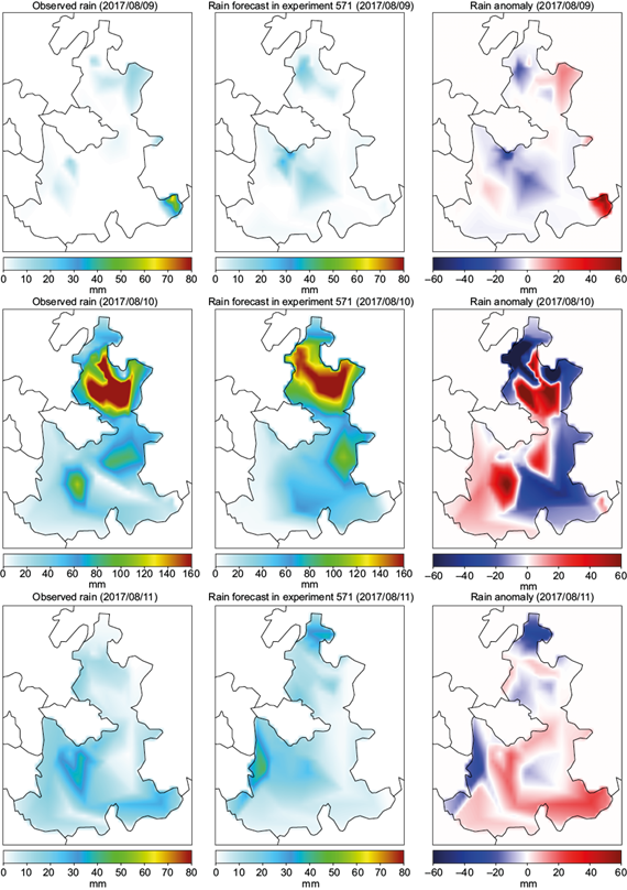
Finally, Figure 9 shows the spatial distribution of the observed and simulated precipitation in experiment 571, together with its corresponding anomaly for August 9, 10 and 11, 2017. On day 10, the highest rainfall of the study period occurred in the northern region of the state of Puebla, associated with Hurricane Franklin. It was observed that the WRF model had the ability to simulate the intensity of precipitation during the extreme event; however, rainfall patterns show variations in detail. These variations are mainly associated with the fact that the 8-km resolution of the model in the nested domain was insufficient to characterize the terrain in the complex topography of the state.
4. Discussion
The performance of the mesoscale models is sensitive to physical parameterization schemes, so it is necessary to perform several experiments with different combinations (Das et al., 2015). In this context, the relevance of evaluating the WRF model with different physical settings for the state of Puebla is evident, especially before the possible implementation of the model in an operational way for the issuance of meteorological alerts, the implementation of early warning systems, or the undertaking of studies. Otherwise there is a risk of obtaining values that do not represent the real or approximate precipitation behavior, and significant errors in the forecast will hinder the prevention and analysis of natural disasters.
In correspondence with the works of Ochoa et al. (2015) and Wu et al. (2016), it is highlighted that the WRF model can reproduce individual peaks of precipitation, thus allowing to analyze the evolution of intense precipitation events in the study area, such as those observed on August 10 in the north region of the state of Puebla, originated by the passage of Hurricane Franklin. On the other hand, Lekhadiya and Jana (2018) mention that the WRF model can very well represent the cloud pattern and spatially recognizes rain events, but that it overestimates the determination in the six parameterization schemes evaluated in their study.
The results in this study point out that the WRF model has the capacity to achieve a high performance for precipitation forecast in specific locations in the state of Puebla, attaining very high positive correlations with values of up to 0.98 at the OYAPB, ZCPPB, and ZRGPB stations, a limited significant cumulative bias of ± 0.01 in 41 of the observation sites (76%), and a low intensity RMSE with values below 3.18 mm at ACHPB and TPYPB stations. However, the optimal configuration of the model in one location does not offer the same level of performance in other observation sites. This result corresponds to Jankov and Gallus (2005), who evaluated the impact of 18 different combinations of physical settings and their interaction with the precipitation of mesoscale convective systems, concluding that none of the scores obtained with the evaluation metrics applied (correspondence relationship and squared correlation coefficient) in the18 combinations was the best for all times and thresholds. However, in this study, by selecting experiment 571, which obtained the highest EMI value, it was shown that it is possible to obtain acceptable results at the state level.
5. Conclusions
In compliance with the first objective of this work, the results of the quantitative evaluation of the WRF model performance for simulating rainfall in the state of Puebla, allowed us to determine that it is possible to configure the model to obtain high performance per observation site and acceptable performance statewide.
Of the 54 observation sites, only the TEZPB station had unsatisfactory results with respect to the Pearson correlation, which obtained a maximum of 0.06 in experiment 456, and a high RMSE with a value of 25.54 in experiment 597. However, for this location, an acceptable bias was obtained with a value of -0.01 in experiment 131.
The application of the Efficiency Multiparameter Index allowed the determination of experiment 571 as the optimal configuration of the WRF model for a statewide application. In addition, after analyzing the 10 best configurations according to the EMI, it was identified that the settings of the microphysics WRF Single-Moment (WSM) 5-class scheme (option 4), the convection parameterization Grell-Devenyi ensemble scheme (option 3), the planetary boundary layer parameterization Mellor-Yamada-Janjic (Eta) TKE scheme (option 2), and the long wave radiation Goddard Shortwave Scheme (option 2), should remain constant to achieve acceptable and uniform performance at the state level.
It should be noted that, in general, the WRF model has a better performance at altitudes greater than 2000 masl, especially in the northern and central regions of the state of Puebla, while in latitudes below 1000 masl, mainly in the south and southeast regions of the state, the model performance is below the state average.
The social relevance of this study lies in the fact that the northwest region of the state of Puebla presents a high risk of flooding due to the rainfall characteristics of the area and the occurrence of tropical cyclones. During the study period, the rainfall reported on August 10 due to the occurrence of Hurricane Franklin exceeded the historical maximum according to official CONAGUA records, with values of 225, 281 and 198 mm at SOLPB, ZCPPB, and Zaragoza ZRGPB stations, respectively. For this same day, the rainfall simulated with the WRF model reached values of 198/187/208/196 at the SOLPB station, 207/245/226/201 at the ZCPPB station, and 126/106/126/126 at the ZRGPB station in the four best cases exposed by location, that is, the cases with lower BIAS and RMSE, and higher r and EMI at the state level. These results indicate that running the WRF model with the optimal configuration will allow to anticipate the magnitude of precipitation events in the state of Puebla with a high degree of precision. Also, with the intervention of an experienced weather forecaster, it is possible to obtain reliable precipitation forecast advisories and bulletins. This will allow authorities, companies and citizens to mitigate or even prevent catastrophic damage caused by extraordinary precipitation.
Additionally, the differentiated signal between bias and RMSE in the best experiments for each observation site, indicates that in the simulation of precipitation in the state of Puebla, the WRF model does not present systematic errors that can be adjusted directly by linear regression. That is, the errors occur randomly, associated with the chaotic behavior of the atmosphere.
Finally, as future work, it is proposed to apply the methodology presented in this research to calibrate the WRF model at the national level.

