


 nueva página del texto (beta)
 Inglés (pdf)
 Artículo en XML
 Referencias del artículo
 Enviar artículo por email
 Citado por SciELO
  Similares en
SciELO
Similares en
SciELO 
 Permalink
1. Introduction
Evapotranspiration (ET) is a fundamental ecosystem process that transfers large amounts of water from the surface to the atmosphere via soil evaporation (E) and plant transpiration (T) (Shuttleworth, 2006; Kool et al., 2014). ET is a combined flux largely related to the Earth energy balance, and strongly controlled by the vegetation structure and physiological processes (Jasechko et al., 2013; Wang et al., 2014). Water is transferred to the atmosphere from soil moisture surfaces and plant leaves (but not solely) pools. T is the loss of water from plants through stomata pores which open during photosynthesis and stomatal opening links the water and C cycles in terrestrial ecosystems (Nobel, 2009). Stomatal conductance is a measure of the rate of flux of either water vapor or CO2 through stomatal pores (Nobel, 2009). Therefore, there is a link between ecosystem productivity and water fluxes commonly studied as water-use efficiency (Huxman et al., 2005; Seibt et al., 2008; Eamus et al., 2013).
Arid and semi-arid regions represent 45% of the terrestrial surface and in these regions, ET is over 80% of the total precipitation (Chapin et al., 2002; Biederman et al., 2016). Despite that the ratio of T to ET (T/ET) is highly variable. There is a tendency for T to be the dominant flux, especially in semi-arid ecosystems due to their dependency on water (Reynolds et al., 2000; Yépez et al., 2007; Raz-Yassef et al., 2010; Vivoni, 2012). A worldwide review by Schlesinger and Jasechko (2014) showed that T can represent 61% of ET in different types of ecosystems, and around 51% in many shrublands and deserts.
Ecosystems where a larger proportion of ET comes through T (high T/ET ratio) will be more productive than those with a low T/ET (Huxman et al., 2005; Ponce-Campos et al., 2013). Nevertheless, there is little information that provides empirical estimates of T/ET at ecosystem scales (Newman et al., 2006; Raz-Yassef et al., 2010; Jasechko et al., 2013; Schlesinger and Jasechko, 2014; Stoy et al., 2019) and its relation to carbon fluxes (Scott et al., 2006; Yépez et al., 2007; Ponce-Campos et al., 2013), which limits our understanding of ecohydrological processes of arid and semi-arid ecosystems (Newman et al., 2006).
Techniques to measure ET have improved significantly to address questions regarding ecosystems functioning and water balance (Shuttleworth, 2006; Kool et al., 2014; Stoy et al., 2019). Modeling approaches are also commonly used to provide information about T and E estimates (Reynolds et al., 2000; Méndez-Barroso et al., 2014; Kool et al., 2014). Although modeled estimates of ET components are useful to account for water budgets, field validation data are needed to refine models at the appropriate scales.
A few techniques exist to partition ET in its components; yet the fundamental problem is the spatial representation to separate measurements of E or T at a consistent scale with ecosystem studies. For example, leaf chambers or porometer techniques allow estimation of T on a single leaf (Wang and Yakir, 2000); sap flow methods determine T of individual trees; soil E can be estimated using flow chambers positioned above the soil surface (Raz-Yaseef et al., 2010), or with lysimeters that estimate E by accounting changes in soil water content (Wenninger et al., 2010). However, the error propagation when scaling these methods to an entire ecosystem is substantial (Wilson et al., 2001; Kool et al., 2014). The eddy covariance technique (EC) provides a direct and continuous estimate of ET within an ecosystem and does not directly distinguish the contributions of its individual components (Li et al., 2019). Recent studies have been able to partition ET via water-use efficiency as the ratio of gross primary productivity (GPP) and ET (Zhou et al., 2016; Scanlon and Kustas, 2010). However, large uncertainties are associated to the estimation of GPP, which is not measured but modeled (Reichstein et al., 2005), which is an important issue for the partitioning of ET (Tarin et al., 2020). Therefore, the study of ET and its components demand a combination of techniques (Williams et al., 2004; Raz-Yassef et al., 2009; Stoy et al., 2019). Combining EC and stable isotope techniques is an alternative that allows ET partitioning ecosystems-scales (Williams et al., 2004; Yépez et al., 2007; Good et al., 2012; Tarin et al., 2014). This is possible since the stable isotopes of water can be used as tracers of the hydrological cycle due to their different fractionation processes that are predictable using parameters such as temperature and humidity (Yakir and Sternberg, 2000).
In this study, we aimed to estimate the fraction plant T that corresponds to the total ET flux (T/ET) in a semi-arid ecosystem in the northwest of Mexico. The northwest hydroclimate of Mexico is strongly controlled by the North American Monsoon (NAM) system (Watts et al., 2007; Vivoni et al., 2008), which delivers most of the annual precipitation during the warm summer from June to September (Lizárraga-Celaya et al., 2010). Thus, semi-arid ecosystems in the northwest of Mexico are highly depend on water availability. We used isotopic measurements of water samples from stems, soils and atmospheric vapor in a multi-species ecosystem and continuous measurements of ET from the EC method. We considered the contribution of multiple species for the estimation of the isotopic composition of T (δ T ) at an ecosystem-scale. Therefore, the specific objective was not only to compare and test different approaches for estimating T/ET using the stable isotope technique, but also to incorporate a weighting of the species-specific physiological traits such as stomatal conductance and the relative plant cover in the final estimation of δ T , which has not been previously assessed for this application.
1.1 Stable isotope: theory
The stable isotope ratio of an element is represented by the notation δ, which relates measured values to a standard as: δ = [(R sample /R standard ) -1]×1000, where R sample and R standard are molar ratios of heavy isotopes over light isotopes (2H/1H and 18O/16O) present in a sample and the standard mean ocean water (SMOW), respectively (Ehleringer et al., 2000). The δ value is in units of parts per thousand (‰). The isotopic model to estimate the ratio of T to ET is fundamentally based on a mass balance approach (Yakir and Sternberg, 2000):
where T/ET represents the ratio of T to total ET flux; δ ET is the isotopic composition of ET which is determined by the Keeling plot approach using isotopic measurements of water vapor and vapor concentrations within a gradient (Wang and Yakir, 2000); is the isotopic composition of T, and δ E is the isotopic composition of the vapor from E (Craig and Gordon, 1965).
The fundamental concept of the Keeling approach is that there are only two different sources of water to ET and this allows the identification of the isotopic composition of the source ET flux, δ ET (Wang and Yakir, 2000; Pataki et al., 2003; Wang et al., 2015). Traditionally, the isotopic composition of water vapor has been monitored using a cold trap method (Helliker et al., 2002), while recent studies have used laser spectroscopy systems (Wang et al., 2010; Griffis, 2013; Good et al., 2014; Sun et al., 2014). Even though laser spectroscopy technology with a resolution of one second is commercially available, there are several problems that have not been resolved yet. For example, the real-time method requires a gradient of moisture (Wang et al., 2015), and robust calibrations have to be implemented continuously with a known isotopic composition during the measurements in laboratory or field experiment (Rambo et al., 2011; Good et al., 2012).
The Craig and Gordon (1965) model can be applied to estimate the isotopic composition of E (δ E ) using the isotopic composition of soil water as:
where δ L is the isotopic composition of liquid water at the evaporating front in the soil (usually 0.05 to 0.1 m depth); δ a is the isotopic composition of the background atmospheric water vapor (0.1 m above the soil surface); α* is an equilibrium fractionation factor that is temperature dependent [α* = (1.137 (106/T soil 2 ) - 0.4156 (103/T soil ) - 2.0667)/1000 + 1] with T soil in degrees Kelvin (Majoube, 1971); ε* = (1-α*) × 10-3; ε k is the kinetic fractionation factor for oxygen (1.0189 in a static boundary layers; Merlivat, 1978); and h is the relative humidity normalized to the temperature of the soil surface. In general, Eq. (2) calculates how evaporating vapor is depleted in heavy isotopes relative to the evaporating water body (soil water moisture). Depletion of the heavy isotope occurs because the lighter isotope diffuses faster than the heavier isotope.
Contrary to the estimation of δ E and δ ET , δ T can be estimated in different ways. The simplest way is to assume that T occurs at an isotopic steady state (ISS), where the isotopic composition of water in stems (in this case the source of water; δ s ) is assumed to be the same as the water being transpired by the canopy (Yakir and Sternberg, 2000; Yépez et al., 2003). This condition is in fact possible since plants do not accumulate heavy or light isotopes and should be valid at daily timescales. However, at an instantaneous-scale, plants may not transpire at steady state due to transient changes in atmospheric conditions and the physiological state of the plants, for example regulation of stomatal conductance (Farquhar and Cenusak, 2005). In order to calculate a δ T value in isotopic non-steady state (NSS) conditions, we can first model the isotopic composition of water at the sites of evaporation following Farquahar and Cenusak (2005) and then apply the Craig and Gordon model (Eq. [2]). Measurements of isotopic composition of leaf water at the sites of evaporation are, however, extremely difficult. Due to the bulk leaf, water often does not represent the actual water that is being transpired and, instead, it is a mixture of unfractionated water from leaf veins that do not evaporate, and heavily fractionated water at the evaporation sites (Farquahar and Cenusak, 2005; Wang et al., 2015). However, an alternative to approximate a reasonable value of leaf water isotopic composition under NSS conditions is given by the Dongmann et al. (1974) model:
where δ en (T) and δ en (T-1) are the NSS compositions of the leaf water at time t and at time (T-1), respectively; ∆t is an interval time in seconds; and δ es (T) is the isotopic steady state composition of leaf water at time t based on (Yakir and Stenberg. 2000):
where δ s is the isotopic composition of the stem water and δ ss is the isotopic composition of bulk leaf water at ISS. The term p is the Péclet number determined as (T leaf • L)/(C • Dw), where C (55.5 × 10³mol m-3) is the density of water, Dw (m2 s-1) is the diffusivity in water of a given species, L (m) is the scaled length over which liquid phase diffusion occurs and T leaf (mol m-2 s-1) is the leaf T rate (Farquhar and Cernusak, 2005). The isotopic composition of bulk leaf water at ISS is obtained as:
where δ a represents the isotopic vapor near the canopy; ε k is the kinetic fraction in the laminar leaf boundary layer; and h is the relative humidity value at the leaf surface temperature. In Eq. (3), Δt is a time interval in seconds and τ = W/T leaf represents the turnover time of water in the leaf, where W (mol m-2) is the molar concentration of leaf water. The term ς relates α* α k (1 - h) where α k is the kinetic fraction factor (1.023; Cappa et al., 2003) and α* and h are as in Eq. (3). Thus, the isotopic composition of T at non-steady state (NSS) conditions can be estimated by replacing δ L with δ en (t) in Eq. (2), to obtainδ T,NSS .
Although δ ss does not estimate the isotopic enrichment at the sites of evaporation, it does represent the instantaneous condition of the leaf water and therefore is useful to represent the isotopic changes at the leaf through time (Flanagan and Ehleringer, 1991; Farquhar and Cernusak, 2005; Lai et al., 2006; Farquhar et al., 2007). Thus, the non-steady state model values of transient leaf water enrichment are a robust approximation of the isotopic composition of leaf water to estimate δ T . Several studies have discussed the importance of accounting an NSS approach to determinate δ T for ET partitioning studies. For example, Xiao et al. (2012) and Wang et al. (2015) have concluded that complex models (e.g., NSS models considering the Péclet effect) do not necessarily add precision to estimates of δ T in canopy level studies, since the consideration for the NSS assumption affecting estimates of δ T mainly depends on the time-scale of interest (Cernusak et al., 2016).
1.2 Proportional contribution of species to
In this study, we proposed an alternative to estimate δ T in a multi-species ecosystem. To illustrate this approach, δ T will be estimated using three different methods: (1) as a simple average of the δ s of the contributing species hence assuming T at steady state conditions to give δ T,ISS ; (2) as a simple average of δ T,NSS (accounting for the Péclet effect), which is obtained by replacing δ L in Eq. (2) with values from δ en (t) for each species (δ T,NSS(sp) ); and (3) as in δ T,NSS , but accounting for the relative importance (RI) of each species based on stomatal conductance and plant cover fractions (δ T,RI ).
The later approach introduced here considers the stomatal conductance fraction of each species relative to the sum of the stomatal conductance values of all species (g f ) and (c f ), which is the canopy vegetation fraction based on the relative aerial canopy cover of each species. The relative contribution of δ T,NSS(sp) to δ T was determined as:
and involves weighting the isotopic composition of each species (sp) with the product of their contributions to total canopy cover (c fi ) and stomatal conductance (g fi ) for the n number of species considered. This leads to a weighted average accounting for the relative importance of each species in (δ T,RI ).
2. Material and methods
2.1 Study location
The study site is a subtropical shrubland near the town of Rayón, Sonora at coordinates 110.53º W, 29.74º N at ~ 630 masl, and it is part of the MexFlux network (Vargas et al., 2013; Villareal et al., 2016). The climate of the region is semi-arid BSh according to Köppen’s classification (Verduzco et al., 2018). Historical mean annual temperature is 21.4 ºC and the precipitation is about 515 mm, with temperatures above 40 ºC in summer and temperatures ranging between 0 and 15 ºC in winter. Dominant species are Fouquieria macdougalii, Acacia cochliacantha, Parkinsonia praecox, Mimosa distachya, Jatropha cordata, and Prosopis velutina. The shrubland is influenced by precipitation of the NAM (Watts et al., 2007), which brings about 60% of the annual precipitation. For this reason, most of the species at the site lose their leaves in the dry season (from October to June) and recover their greenness in late June or early July. Several hydrological and eco-hydrological studies have been conducted in this site (Vivoni et al., 2010; Méndez-Barroso et al., 2014; Tarin et al., 2014; Verduzco et al., 2018).
Vegetation cover was estimated using seven transects of 100 m in length around a central point marked by a flux tower. In these transects cover percentage was estimated by summing the aerial canopy of each species crossing the transect relative to the length of the transect. Vegetation height was between 2 to 5 m with a sparse cover that can reach a maximum leaf area index (LAI) of 1.7 based on the Moderate Resolution Imaging Spectroradiometer (MODIS) product at 500 m. The Normalized Difference Vegetation Index (NDVI) for the site was obtained from MODIS at 250 m, which detects changes in vegetation greenness.
2.2 Instrumentation
A 9 m tower was installed in the subtropical shrubland to make long-term meteorological and eddy covariance measurements of ET as described in detail by Verduzco et al. (2018). In brief, the system consisted of an open path LI7500 infrared gas analyzer that provides simultaneous measurements of both water vapor and carbon dioxide (LI-COR, Lincoln, NE) and a three-dimensional sonic anemometer (CSAT3, Campbell Scientific, Logan, UT) that sampled the atmosphere at a frequency of 10 Hz using a CR5000 datalogger (Campbell Scientific). Fluxes were calculated at 30 min averaging periods considering typical rotation and density corrections as shown by Scott et al. (2004). Other sensors at 30 min resolution were installed to measure net radiation (NR-LITE-L, Campbell Scientific), air temperature and relative humidity at 0.1, 2.5, 4.5 and 9 m above the ground (HMP45D, Vaisala, Helsinki, Finland) and wind speed and direction (Wind Monitor, Young, MI). Soil moisture (θ) was measured at 0.05 and 0.3 m depths with two water content reflectometers at the tower (CS616, Campbell Scientific) and precipitation was measured with a tipping bucket rain gauge (TR-525USW, Texas Electronics, Dallas, TX). These data were also averaged over 30 min intervals, except for precipitation (half-hour sums) and were logged using a CR-23X datalogger (Campbell Scientific). Energy closure was determined using least squares comparison from fluxes: latent heat (LE), sensible heat (H), ground heat (G), and net radiation (Rn). Regressions between turbulent fluxes of (H + LE) against (Rn - G) for all summers had a slope of 0.75 (± 0.04; p-value < 0.005), and intercept of 16 (± 2) W m-2, a coefficient of determination (R2) of 0.93 (± 0.005; p-value < 0.001) and an energy balance of 0.83 (± 0.02; p-value = 0.034) (Méndez-Barroso et al., 2014). Potential evapotranspiration (ETP) was estimated following Garatuza-Payán et al. (1998). The relative water content (RWC) was estimated using the measurements of θ relative to a saturation value of 40%.
2.3 Soils and stems sample collection
This study encompasses two years (2007 and 2008) during the NAM season. Field campaigns were performed in different days of the year (DOY) in dry periods (July 22, 23 and 24: DOY-203, DOY-204 and DOY-205 for 2007; July 3 and 4: DOY-185 and DOY-186 for 2008), and wet periods (July 27: DOY-208 for 2007; July 14 and 15: DOY-196 and DOY-197 for 2008). Sample collections for isotopic analysis were atmospheric water vapor, soil, and stems. Water vapor was collected using the cold trap method in all study days and clustered in periods. To get a vapor concentration and isotope gradient for Keeling plots, water vapor was caught at corresponding heights of temperature and humidity measurements (0.1, 2.5, 4.5 and 9 m). Water vapor was simultaneously collected every two hours from all heights with an automatic cryogenic trapping system (Yépez et al., 2003), which pulled air through low-absorption tubing attached to the tower. Glass traps were submerged in a -80 ºC alcohol bath over a 30 min collection period (Helliker et al., 2002). Flow rate was regulated to 500 ml min-1 to collect from 30 to 50 µL of water in each glass trap.
Stems were collected in four dominant species at the subtropical shrubland: Fouquieria macdougalii, Acacia cochliacantha, Parkinsonia praecox, and Prosopis velutina (n = 3 per species). Stem samples were placed in glass tubes and immediately sealed with Parafilm® to avoid water evaporation. Soil samples were collected from 0.05 to 0.1 m depths in two different microsites at bare soil and under canopies for a total of six samples per microsite on each collection day.
Water from soils and stems was extracted at the laboratory using the cryogenic distillation method described by West et al. (2006) accepting extractions that confirmed that more than 95% of the water by weight was obtained. Water samples were analyzed in a cavity ring-down spectroscope (DLT-100, Los Gatos Research, Mountain View, CA). The accuracy of the isotope analysis was 0.4‰ in 18O with respect to the LGR standards #1 and #5 from Los Gatos (LGR, 2008).
2.4 Estimates of the isotopic composition of T, E and ET
Using the measurements of temperature and relative humidity, we estimated the atmospheric moisture concentration at different heights as the water vapor was collected. The inverse of the water content (1/mg H2O m-3 of air) was plotted in x-axis, while water vapor isotopic composition was plotted in y-axis to produce Keeling plots (Wang and Yakir, 2000). The y-intercept of the best linear fit of these plots was used to obtain δ ET .
We averaged the isotopic composition of soil water (δ L ) to obtain a single value for the δ E calculation each day (Eq. [2]). The isotopic composition of the stem water (δ s ) was used to estimate the isotopic composition of T (δ T ) with three different approaches as follows:
δ T,ISS in ISS, with a simple average of the isotopic composition of the stem water of four different species δ T,ISS = 1/n ∑δ s .
In NSS modeling (Eqs. [3], [4] and [5]), δ T with Craig and Gordon (1965) was calculated using δ en (t) for the four species, to produce δ T,NSS(sp) and then with the average to obtain δ T,NSS in the same interval of the Keeling plots;
In NSS but adding the relative isotopic contribution (RI) value δ T,RI(sp) to obtain δ T,RI (section 1.2).
To estimate g f we measured stomatal conductance in four individuals of all four species during periods corresponding to water vapor trapping with a porometer (SC-1 Leaf Porometer Systems, Decagon Devices, Pullman, WA). For each species, c f was adjusted to 100% based on the percentage cover of the four representative species: F. macdougalii represents 21%, A. cochliacantha 16%, P. praecox 10%, and P. velutina 18%. To estimate the turnover time of leaf water (τ in Eq. [3]) we used estimates of leaf transpiration (T leaf ) determined in each species using stomatal conductance values related to vapor pressure deficit. The W value to calculate the turnover time of water in the leaf were 5.3, 9.8, 10.9, and 6.1 (mol m-2) for A. cochliacantha, P. praecox, F. macdougalii, and P. velutina, respectively (Tarin et al., 2014). Thus, τ was calculated as the difference between T leaf and W (Eqs. [3] and [4]). In Eq. (5), the kinetic fraction (ε k ) was given by ε k = (32r s + 21r b )/(r a + r b + r s ), applied for δ 18 O (Wang et al., 2015). To estimate the stomatal resistance (r s ) at the daily scale, we used the relation of stomatal conductance and vapor pressure deficit. Aerodynamic and boundary-layer resistance values, r a and r b (in mol m-2 s-2), were 3 and 1, respectively. The time interval used in Eq. (3) was 1800 seconds, and 0.008 m was used for L in the Péclet number.
2.5 Estimation of T/ET and uncertainties
The mass balance calculation of T/ET was applied using the three different approaches to calculating δ T in Eq. (1). To calculate the volume of water transpired by vegetation, we used the values results from the T/ET derived from δ T,RI (T/ETIR). Fraction values of T/ETIR were multiplied by the daily total ET that was continuously measured with the eddy covariance technique in mm d-1.
The uncertainty in the estimation of T/ET (for the three approaches) was determined using the error propagation tool developed by Phillips and Gregg (2001). This method is based on the standard error of the source proportions and mixing, which considers the errors in the y-intercept from Keeling plots for δ ET , standard deviations, standard errors and sample size of the sources (δ E and δ T ).
3. Results
The monsoon season started between DOY 180 and 190 in both years. Each year had different inputs of precipitation during the NAM (Fig. 1d-h) with 2008 being significantly wetter than 2007 (Table I). Mean daily values of weather showed that 2007 was slightly cooler than 2008 during summer conditions (Table I). However, vapor pressure deficit, wind direction and wind speed were similar for both years.
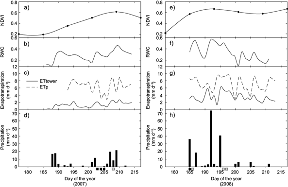
Fig. 1 Environmental conditions of the subtropical shrubland during the North American Monsoon season for 2007 and 2008. (a) and (e) 16-day NDVI composites; (b) and (f) relative soil water content (RWC) at 0.05 m depth; (c) and (g) ET estimated by the EC technique (ETtower) and potential ET (ETp); (d) and (h) precipitation. Black squares at the bottom of the figure indicate dry days of measurements while grey squares denote wet days of measurements.
Table I Weather and climate conditions for 2007 and 2008 during the study period (DOY-185 to DOY-220).
| Variable | Daily average | |
| 2007 | 2008 | |
| Rain (mm) | 143 | 199 |
| Tair (ºC) | 22.4 (± 2.2) | 27.0 (± 1.8) |
| RH (%) | 51.5 (± 13.4) | 66.1 (± 9.5) |
| VPD (kPa) | 1.8 (± 1.2) | 1.6 (± 0.5) |
| WS (m s-1 ) | 1.7 (± 0.3) | 1.6 (± 0.5) |
| WD (º°) | 205.4 (± 25.7) | 191.0 (± 26.8) |
| Tair (max; ºC) | 26.9 | 30.4 |
| Tair (min; ºC) | 18.9 | 23.8 |
| VPD (max; kPa) | 2.54 | 2.19 |
| VPD (min; kPa) | 0.6 | 0.5 |
Tair: air temperature; VPD: vapor pressure deficit; WS: wind speed; WD: wind direction.
Maximum daily and minimum values of air temperature and VPD as Tair max and Tair min, VPD max and VPD min, respectively.
In 2008, the maximum precipitation event was of 73 mm d-1, while in 2007 maximum precipitation was 20 mm d-1. Precipitation had a significant effect on ET. During the period between DOY-180 to DOY-215 in 2007, ET represented 30% of precipitation (total = 119 mm), while during the same period in 2008 with 80 mm more of precipitation, ET represented 50% of the total precipitation. In 2008, maximum ET value was 5.9 mm d-1, in contrast to 2007 that had 2.7 mm d-1. Peak values of ET occurred over a short period (Fig. 1c, g), with a small delay after each precipitation pulses.
The RWC in 2008 was over 0.50, whereas in 2007 it showed a maximum value of 0.45 in DOY-209. These differences among years showed the influence of precipitation on ET flux. NDVI was similar in both years, but the maximum NDVI value in 2007 was 0.61 in DOY-209, while in 2008 the maximum NDVI value was 0.67 in DOY-193 due to early precipitation prior to the study period (rainfall during DOY-179 was 14.6 mm d-1).
3.1 Isotopic composition of ET and E
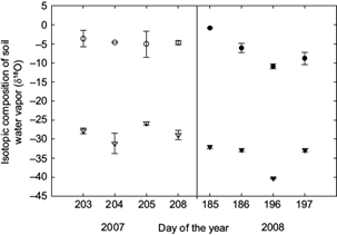
Keeling plots determined the isotopic composition of ET (Table II). δ ET was more enriched during dry periods in both years compared to wet periods. We observed that for the three days of the dry period in 2007, values of δ ET were between 0 to -10‰ δ 18 O (Table II). In contrast, during the wet period in 2007 (DOY-208), after a precipitation pulse of 20 mm d-1 (Fig. 1), δ ET was depleted in heavy isotopes (Table II) showing a value of -18.91‰ δ 18 O. In the same way, during dry periods in 2008, δ ET had enriched values in the order of 7 to -3‰ δ 18 O, but on DOY-196, when precipitation pulses started, we observed δ ET as depleted as -25.53‰ δ 18 O.
Table II Regression parameters for Keeling plots of water vapor.
| Year | DOY | Sampling times | n | R2 | Slope | s | Intercept (δ ET ) | s |
| 2007 | 203 | 7-16 h | 11 | 0.43** | -2.5 E + 02 | 9.5 E + 01 | -0.60 | 6.1 |
| 204 | 7-11 h | 7 | 0.15 | -1.5 E + 02 | 1.6 E + 02 | -5.60 | 9.7 | |
| 205 | 8-17 h | 20 | 0.66* | -1.8 E + 02 | 3.0 E + 01 | -7.13 | 1.7 | |
| 208 | 7-17 h | 16 | 0.40* | 6.0 E + 01 | 2.0 E + 01 | -18.91 | 1.1 | |
| 2008 | 185 | 17-18 h | 4 | 0.81*** | -2.8 E + 04 | 9.4 E + 04 | 7.53 | 7.1 |
| 186 | 7-12 h | 8 | 0.61** | -1.7 E + 04 | 5.4 E + 04 | -3.89 | 3.3 | |
| 196 | 7-11 h | 7 | 0.38 | 6.0 E + 04 | 3.5 E + 04 | -25.53 | 2.0 | |
| 197 | 8-11 h | 8 | 0.61** | -8.2 E + 04 | 2.6 E + 04 | -16.32 | 1.6 |
s: standard error; *, ** and *** mean statistical significance with 99%, 95% and 90%, respectively.
In both years, we noted that evaporated water from the soil was significantly depleted in heavy isotopes with respect to δ L , showing a difference on the order of 20‰ to 30‰ δ 18 O (Fig. 2). In 2008, we observed depletion in δ L reaching values above to -10‰ in DOY-196. δ E values tended to be lighter in this period. There were no differences in δ E estimates between years: in 2007, δ E showed values around -23‰ ± 2.4 δ 18 O, while in 2008, δ E showed values in the range of -28‰ ± 3.2 δ 18 O.
3.2 Isotopic composition of transpiration
Our methods to estimate the isotopic leaf water enrichment at ISS and NSS did not show significant differences in the first hours (from 6 am to 10 am) of the day for the four species considered (Fig. 3 only DOY-196 is showed). After 10 am, the difference between ISS and NSS increased from 1‰ to ~5‰ δ 18 O. Prosopis velutina showed the largest difference with 6.15‰ in the evening, followed by Fouquieria macdougalii with 4.7‰, Acacia cochliacantha with 4.1‰, and Parkinsonia praecox with a difference of 2.14‰ δ 18 O. These small differences between NSS and ISS have major implications in the estimation of δ T (Eqs. [2] and [3]), meaning that δ T stayed moderately constant through the day. Ultimately, whether δ T changes during the day or not, it may affect the T/ET partitioning, as it is explained next.
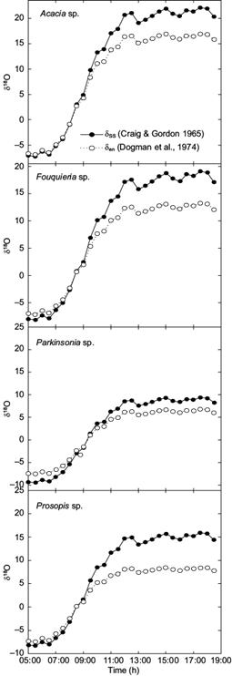
Fig.3. δ 18 O-enrichment of leaf water (‰) of representative species of a subtropical shrubland on DOY-196 of 2008. δ ss is the predicted enrichment at isotopic steady state, δ en is the leaf enrichment under isotopic non-steady state conditions.
Values for the different approaches to estimate δ T (δ T,ISS , δ T,NSS and δ T,IR ) showed enriched values in both years (Fig. 4). Particularly in 2008, these were considerable higher in heavy isotopes with values from 2.56 to 8.54‰ δ 18 O, while 2007 showed values from-3.9 to 8.23 ‰ δ 18 O. Differences between the methods δ T,ISS and δ T,NSS were more significant in DOY-203 (2007) and DOY-186 (2008); however, these days also showed the larges uncertainties ranging between ± 2.92 and ± 12.91‰. In contrast, differences in δ T,ISS and δ T,IR were ~4.1‰ δ 18 O, and standard errors of both estimates overlapped in the eight days of this study (Fig. 4).
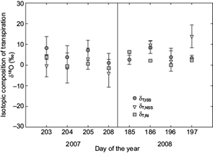
Fig. 4 Isotopic composition of transpiration for key species of the subtropical shrubland, using three different methods: (1) δ T,ISS is the average isotopic composition of stem water, (2) δ T,NSS is the modeled isotopic composition of transpiration with the isotopic non-steady state approach, and Péclet effect; and (3) δ T,RI is considering non-steady state conditions and weighting factors of stomatal conductance and vegetation cover fractions. Symbols are means ± standard errors.
3.3 Evapotranspiration partitioning
With the estimation of T/ET using the three approaches to calculate δ T in Eq. (1), we found that a maximum uncertainty of 30% in the final estimate of T/ET if using δ T,IR (Table III). However, the statistical error of the three methods of T/ET fall within the variation expressed by the error propagation (Phillips and Gregg, 2001) and generally overlapped with the simplest approach T/ET(ISS) (Table III).
Table III T/ET partitioning using three different approaches: T/ETISS using δ T from δ ISS , T/ETNSS using δ NSS modeled with Craig and Gordon (1965) and T/ETRI considering RI in isotopic composition of T (δ RI ).
| Year | DOY | T/ETISS | T/ETNSS | T/ETRI |
| 2007 | 203 | 0.76 (0.18) | 0.99 (0.25) | 0.93 (0.21) |
| 204 | 0.73 (0.29) | 0.86 (0.25) | 0.78 (0.29) | |
| 205 | 0.57 (0.07) | 0.65 (0.09) | 0.62 (0.06) | |
| 208 | 0.33 (0.05) | 0.40 (0.08) | 0.35 (0.05) | |
| 2008 | 185 | 1.00 (0.24) | 1.00 (0.18) | 1.00 (0.19) |
| 186 | 0.70 (0.08) | 0.78 (0.13) | 0.74 (0.09) | |
| 196 | 0.33 (0.05) | 0.35 (0.06) | 0.35 (0.05) | |
| 197 | 0.46 (0.05) | 0.35 (0.07) | 0.44 (0.08) |
Values in brackets are uncertainties in accordance with Phillips and Gregg (2001).
In 2007, we observed that on DOY-203 and DOY-204, the T/ET(RI) ranged between 0.78 and 0.93 in the dry period with a maximum uncertainty of ± 0.29, suggesting that T dominated the total flux of ET in those days. In contrast, during the wet period (DOY-208), T/ET decreased to 0.35 with an uncertainty of ± 0.05. In 2008, we observed the same pattern as in 2007, T/ET values during dry periods ranged from 1 to 0.74 and from 0.34 to 0.44 in wet days (with uncertainty of 0.19 and 0.05, respectively). The decrease in error estimations was associated with a decreased vegetation contribution (Fig. 1).
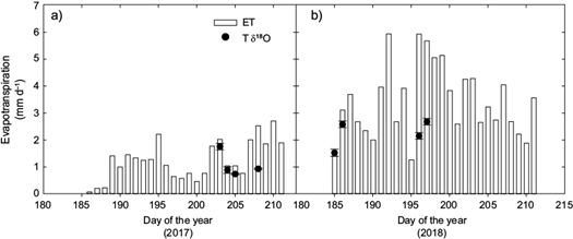
The combination of stable isotopes to calculate T/ET and continuous measurements of ET with the eddy covariance technique allowed us to estimate the volume of water transpired by vegetation (Fig. 5). During DOY-203 in 2007, T/ETRI was of 0.93 ± 0.21 and the total ET was 2.0 mm d-1, meaning that T was ~1.91 ± 0.43 mm d-1. On DOY-202, there was a precipitation pulse of 11 mm (Fig. 1), such that T in DOY-203 represented 20% of the water from the previous precipitation event. For the next two days during this dry period (DOY-204 and DOY-205), ET decreased drastically. ET increased after DOY-207 due to another precipitation event of 20 mm d-1, thus T reached its lowest value of 0.65 ± 0.06 mm d-1 during this period. Similarly, in 2008, T was 80 to 100% of the total ET representing a range of 1.52 to 5.98 mm d-1 during the dry period (DOY-185 and DOY-186; note that DOY-185 was measured previous a big precipitation pulse which occurred at night [Fig. 1]). The wet period had precipitation pulses of 70 mm d-1 in DOY-192 and 40 mm d-1 in DOY-195 and thus, E was the dominant flux over this period (Fig. 5b). On DOY-196 and DOY-197, soil E was 3.86 and 3.17 mm d-1, respectively, while the vegetation greening was at its maximum (Fig. 1).
4. Discussion
The present study provides insights on the variability of the T/ET ratio in a semi-arid shrubland under the influence of the NAM in northwest Mexico. Here we combined stable isotopes of water and the eddy covariance technique using three different approaches for the estimation of the isotopic composition of T (δ T ). We found that E was the dominant flux right after large precipitation pulses (> 40 mm d-1), but T dominated with up to 100% over ET as the relative water content declined. Uncertainties in the final estimate of T/ET increased as the complexity of δ T increased by weighing the proportion of stomatal conductance and vegetation cover for dominant species at the semi-arid shrubland. Our results for this new estimate on δ T in a multi-species ecosystem and implications on eco-hydrological processes are discussed in the following sections.
4.1 Different estimates of T/ET and uncertainties
The novelty of our work relied in the incorporation of physiological and ecological attributes in the stable isotopic approach in a multi-species semi-arid ecosystem. Studies have shown that factors such as vegetation cover, and plant physiological processes, such as stomatal conductance, are important drivers of ecosystem transpiration (Reynolds et al., 2000; Farquhar et al., 2007). Therefore, this study considered the relative importance (RI) of two factors in calculating δ T (stomatal conductance and vegetation cover) in an isotopic non-steady state condition. Results of T/ET using δ T,RI showed that considering non-isotopic steady state conditions and weighting the relative importance of species cover and instantaneous stomatal conductance relative values does not considerably improve the expression of δ T for the mass balance calculation of T/ET (Eq. [1]). These findings are in agreement with previous studies that have shown that a simple steady state is appropriate to calculate T/ET at large spatial-scales, for example at an ecosystem-scale (Xiao et al., 2012; Wang et al., 2015).
A large range of uncertainties was observed (from 5 to 29%) in the final estimation of T/ET with the three methods used (Table III). T/ETIR had the largest errors, but similar to those observed with the simplest approach that averaged the isotopic compositions of water from stems assuming steady state conditions (29%; Table III). Thus, T/ET results tended to overlap regardless of the δ T value used, and this can be explained by the lack of differences between the different calculations of δ T (Fig. 4). Uncertainties in the estimation of T/ET for the subtropical shrubland with multi-species are similar to ecosystems with one or two dominant species, where the magnitude of errors range between 15 to 30% (Yépez et al., 2005, 2007; Xu et al., 2008; Bijoor et al., 2011, Good et al., 2012). However, an uncertainty of almost 30% in T/ET estimation is higher than the 20% observed in a semiarid grassland (Yépez et al., 2005) and riparian woodlands (Yépez et al., 2007). Our findings provide important information for the design of future experiments in multi-species ecosystems since steady state assumptions of transpiration may be reasonable for the estimates of T/ET, which simplifies fieldwork and error propagation significantly.
Large uncertainties in our estimates of T/ETIR may be due to uncertainties and differences within species in stomatal conductance rates. Further studies to compare plant physiological traits of co-existing species can help to better assess plant species contribution over ecosystem transpiration. Additionally, an adequate representation for ecosystems and global studies calls for techniques that, while maintaining ecosystem-level consistency, incorporate for example a better temporal resolution for key contributing parameters to partitioning ET with isotopic methods (Stoy et al., 2019). Real-time monitoring of the isotopic compositions of water vapor with laser spectroscopy are now possible (Wang et al., 2010, 2015; Good et al., 2012; Wei et al., 2019) and can provide dynamic estimates of T/ET that could validate remote sensing and modeling approaches providing information at even larger spatial scales (Nagler et al., 2007; Vivoni, 2012). We thus concluded that scaling up the model complexity in partitioning ET using the stable isotopes approach should merely depend on the addressed question and particular site characteristics. Knowing the T/ET ratio provides important insights about carbon-water relations in terrestrial ecosystem with both hydrological and ecological implications at an ecosystem-scale.
4.2 Ecological implications of T/ET estimates
ET partitioning as the ratio of T/ET across all studied periods ranged from 0.33 to 1.0 (Table III) and this variability can be explained by water availability at the subtropical shrubland. Semi-arid ecosystems such as the subtropical shrubland in northwestern Mexico highly depend on water availability (Verduzco et al., 2018). Trends in T/ET in semi-arid ecosystems have indicated that soil water availability is preferentially used by the vegetation despite that E is expected to be high because of large open areas (Raz-Yaseef et al., 2010) and high ET potential (Heilman et al., 2009; Brooks et al., 2011). Our results are in the same range of empirical estimates of T/ET in other semiarid ecosystems (Ferreti et al., 2003; Huxman et al., 2005; Scott et al., 2006; Nagler et al., 2007; Raz-Yaseef et al., 2010; Wang et al., 2010) and estimates based on ecological and hydrological modelling approaches (Reynolds et al., 2000; Vivoni, 2012; Méndez-Barrozo et al., 2014; Schlesinger and Jasechko, 2014).
Although small precipitation events (< 5 mm d-1) are dominant in semi-arid ecosystems (Loik et al., 2004), climate change predictions suggest that larger events and more pronounced inter-storm periods may become more characteristic (Zhang et al., 2007), particularly for the NAM region (IPCC, 2013). At the subtropical shrubland, total ET was variable among years because of the different inputs in precipitation. ET was lower during the drier year 2007 than in the wetter year 2008. These differences showed contrasting patterns on ET components. E was only briefly dominant when large precipitation pulses in the subtropical shrubland occurred since soil E ratios were ~0.70 of total ET soon after precipitation events (Fig. 5; see DOY-192 and DOY-195 in 2008). However, E rapidly decreased as the soil profile dried down; thus, vegetation transpiration was the dominant component of ET during dry periods and after small precipitation events (i.e., 11 mm DOY-202). These observations are consistent with other studies in ecosystems with sparse semi-arid vegetation cover (Williams et al., 2004; Yépez et al., 2005, 2007; Scott et al., 2006; Xu et al., 2008; Méndez-Barroso et al., 2014). Our comparison between a dry year and wet year and between precipitation size events provides important evidence of how E and T responded to different precipitation amounts.
The T/ET values observed during the monsoon season also had implications on describing ecosystem functioning as controlled by variable precipitation (Huxman et al., 2005). Evaluations of T/ET ratios in terrestrial ecosystems and especially in semi-arid ecosystems are crucial not only for hydrological studies but also for a better understanding of the influence of precipitation over ecological functioning within a changing environment.

