


 nueva página del texto (beta)
 Inglés (pdf)
 Artículo en XML
 Referencias del artículo
 Enviar artículo por email
 Citado por SciELO
  Similares en
SciELO
Similares en
SciELO 
 Permalink
1. Introduction
The high mountain climate is difficult to characterize due to the heterogeneity of its relief. The complex orography in mountain environments leads to different precipitation, insolation and temperature regimes that vary considerably between relatively small distances (Becker and Bugmann, 1997) causing the existence of microclimates and therefore of different ecosystems. The continentality and wind circulation patterns largely govern the precipitation regime, which, in the anabatic region of the mountainous zone, depends on elevation. So at least for the case of the eastern slope of Mexico, within the orographic barrier located between latitudes 18º 45’ and 19º 45’, the area of mesophilic forest (ranging between ~600 and ~2000 masl) has the highest rate of precipitation between the coastal plain and the summits of the eastern high mountains of the Transverse Neovolcanic Axis (Citlaltépetl [5610 masl], Sierra Negra [4580 masl] and Naucampatépetl [4,200 masl]). According to Ortega and Castillo (1996) and Barry (2008), this region experiences an annual precipitation of up to 3000 mm. Above the mesophilic forest, the precipitation regime tends to decrease with elevation; this pluvial decrease is usually more noticeable above the upper timberline (~4000 masl) where the annual accumulated precipitation is generally less than 1000 mm. This pattern of precipitation is common in regions with the incidence of trade winds (Barry, 2008).
As the air masses are forced to ascend, they reach the condensation level of the contained moisture, commonly between 600 and 2000 masl, causing the high accumulated precipitation within this altitudinal range; subsequently air masses continue the ascend with a comparatively drier air (Tejeda-Martínez, 2018). This difference in air relative humidity (%) before and after precipitation is related to the drying ratio (DR) defined as the ratio of precipitation to water vapor influx (Smith et al., 2003). According to Smith et al. (2005), this drying ratio can acquire values from ~20% up to 80% depending on the elevation, having an average value for the mountains of Oregon and California, USA of 43 and 32 %, respectively; in the Alps 35% and in the central Andes reaches an average of ~50% (Smith and Evans, 2007). The Atacama region in Chile has the highest drying ratio in the Americas (Garreaud, 2009). In Mexico this behavior can be noticed in the average annual rainfall of eastern slope weather stations property of the Servicio Meteorológico Nacional (National Weather Service), as well as one station of the Large Millimeter Telescope Alfonso Serrano, in the Sierra Negra volcano (Sierra Negra station) and another of the Geophysics Institute of the UNAM, located in the lower part of the Citlaltépetl glacier (Morrena station). The National Weather Service stations have temperature and precipitation data series ranging in duration from 15 to 100 years, with an average of over 40 years of records. Figure 1 shows a positive trend line between the elevation and the precipitation rate between sea level and ~1800 masl. It also shows that the highest rainfall rate occurs between ~1300 and ~2000 masl. Above this altitude, the precipitation rate shows a negative trend. Despite not belonging to the eastern slope of the country, the Nevado de Toluca weather station is also plotted (green triangle) for comparison, based on its climatological normal data.
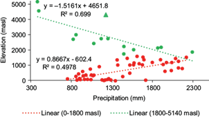
Fig. 1 Altitudinal distribution of precipitation based on stations on the eastern slope of Mexico between latitudes 18º 45’ and 19º 45’. Red circles are stations among 0 and 1800 masl, green circles are stations among 1800 and 5140 masl. For comparison, the green triangle represents the Nevado de Toluca weather station.
In addition to the vertical gradient of tropospheric temperature, which has an idealized behavior of decrease in air temperature with height, the terrain aspect and slope determine the insolation on the surface, which leads to different diurnal temperature ranges (Arya, 2001). According to Geerts (2003)), the frequent arrival of air masses and their condensation favors the frequent cloud formation. Particularly after local noon, it reduces insolation resulting in lower maximum air temperature by ~0.5 ºC for every 2 h of cloudy sky (Harding, 1979).
Other factors indirectly influence the climate of high mountains, such as heat islands produced by large cities. It has been documented that a secondary forcing in the retraction of the glaciers of the volcanoes Popocatepetl (before 1994) and Iztaccíhuatl (5500 and 5220 masl, respectively) is caused by the heat islands of Mexico City, Mexico State and Puebla city (Delgado-Granados, 1996, 1997). This effect of heat islands has also an impact on convective precipitation over the cities that produce them and in the surrounding areas (Ji-Young et al., 2014), including adjacent mountain regions. Morales-Méndez et al. (2007) report this phenomenon in the urban area of Toluca and the surrounding regions. They also state that in addition to temperature, the suspended particles of a certain diameter, as a product of air pollution produced by large cities, cause humidity condensation and increase the rate of precipitation.
Additionally, it has been documented that the alterations in the normal circulation of the Pacific Ocean and the atmosphere (El Niño-Southern Oscillation, ENSO) can modify the precipitation patterns in many regions of the world (Magaña et al., 2003) as well as in mountain regions. This phenomenon is considered in positive phase when the temperature of ocean waters exceeds the average threshold (El Niño), and in negative phase when it falls below the normal range (La Niña). Despite the above, there are oceanic regions that record long-term changes in its surface temperature (Deser et al., 2010). In general, El Niño causes a considerable increase in rainfall in the regions it affects, while La Niña leads to a decrease in the variable. According to Molina (1999), extremely dry regions of Peru and Chile have recorded monsoon-type rains during years of positive ENSO. In the case of Mexico, according to Magaña et al., (1998), there is an increase in winter precipitation in the center of the country during years with an ENSO and lower precipitation during the summer, being opposite during its negative phase. Bravo-Cabrera et al. (2017) emphasize this correlation; however, according to the authors, an increase in the intensity of hurricanes in the Pacific (e.g., Paulina) has been observed during the years of positive ENSO, especially when the Oceanic Niño Index (ONI), in its usual range of -2.5 to +2.5, reaches the highest levels. Periods of ENSO with a high ONI favor the convective action of the humidity coming from the Pacific, which with the apparent weakening of the trade winds (Bravo-Cabrera et al., 2017) generate the increase of precipitation through the Sierra Madre Oriental and mountains of the center of Mexico. Regarding the correlation between the intensity of hurricanes and the positive phases of ENSO, Martínez-Sánchez and Cavazos (2014) found that this relationship is clearer with hurricanes category 4 and 5.
Regardless of the complex task of determining high mountain climates, in Mexico there is a categorization adapted by García (2004) from the Köppen classification. According to the author, in the high mountains of the Sierra Nevada in the center of the country, the “cold climate” starts from 3349 masl with an average annual temperature at that elevation of 8.3 ºC. Above 5272 masl, the "very cold climate" starts with an annual temperature of -1.4 ºC. In the intermediate part, close to 4000 masl (upper timberline), the author states an average annual air temperature of 5 ºC. The lack of pluviometric stations at high altitude prevented the determination of the range of precipitation at these elevations.
With respect to the variability of precipitation and temperature over time, with parameters increasingly farther from their normal values (IPCC, 2013), a large number of investigations have been carried out on a global scale in which the increase of the air temperature is analyzed (IPCC, 2015); while at a local scale, the behavior of precipitation is also studied. However, most of this research at local scale is related to the agricultural industry (Ocampo, 2011) and to the heat islands in major cities mainly (Jáuregui, 1975; Morales-Méndez et al., 2007), because of the change in land use, urban growth and deforestation, among others.
To estimate the variation of temperature and precipitation over time, the Expert Team on Climate Change Detection and Indices (ETCCDI) created 27 indices from daily data (Zhang and Yang, 2004), which can be analyzed according to the requirements of each research and the needs of each ecosystem (Vázquez-Aguirre, 2010). These indices have been used globally to understand the effects of climate variability in recent decades.
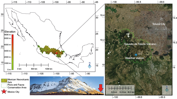
Considering that in Mexico investigations of climatic variation in high mountain areas are limited to correlating the increase in air temperature (Delgado-Granados, 2007), and the surface balance of solar energy (Ontiveros-González et al., 2015) with the retreat of its glaciers, leaving aside other fragile ecosystems (Díaz et al., 2003), in this work we study the main climate change indices at a high mountain environment. Here we analyze the variation in temperature and precipitation variables at the Nevado de Toluca volcano throughout the data series of its weather station (1965-2015). The Nevado de Toluca weather station is the only in situ reference of the high mountain climatic conditions in Mexico with a sufficiently long data series. The elevation at which it is located allows associating the variation of the climate with the ecosystems that predominate above the limit of the continuous forest. It is expected, therefore, that the results of this research will function as a benchmark for high mountain climatic variability, both for the Mexican mountains and for those located in the intertropical region of the planet, where the series of climatic data are shorter or nonexistent.
2. Study area
The Nevado de Toluca or Xinantécatl (“naked man” in Náhuatl language) (19º 09’ N and 99º 45’ W) is a dormant volcano that belongs to the Neovolcanic axis in its central area. It is the fourth highest mountain in Mexico at 4680 masl (INEGI, 2017) located 75 km southwest of the Mexican capital and 23 km from the city of Toluca. Nevado de Toluca is a stratovolcano composed of different evolutionary phases that date from the late Pliocene to the early Holocene; its last eruption occurred 3300 years ago (Macías et al., 1997). It has an elliptical summit of approximately 1.5 × 2 km with the major axis exposed from east to west (García-Palomo et al., 2002). The ease of access allows hundreds of mountaineers to visit the central zone of its crater where the lakes of El Sol and La Luna are located; adjacent to this region, the highest ridges of the stratovolcano are found.
From the year 1936, it was decreed as a National Park and recently in 2013 it was recategorized as a Flora and Fauna Conservation Area with an extension of 53 912 ha, covering 10 municipalities of the State of Mexico. There are 627 species of flora with 52 endemic and nine at risk. The fauna is composed of 175 vertebrate species with 36 endemics; additionally, there are 209 species of fungi. It has great hydric importance since surface runoff on its northern and northeastern slopes supplies the city of Toluca and its conurbation area, as well as part of city of Mexico (Toscana-Aparicio and Granados-Ramírez, 2015). Figure 2 shows the study area and a perspective view of the volcano.
3. Methods
Although the Morrena and Sierra Negra weather stations have been installed at a higher elevation (5140 and 4568 masl, respectively), their time series (2006-2010 and 2014 to date, respectively) are very short and are only used at the institutional level. Therefore, the Nevado de Toluca volcano has the highest elevation publicly available long-term climatological data in Mexico. Its weather station is located at 4283 masl with coordinates 19º 07’ 07” N and 99º 46’ 53” W (station Nevado de Toluca, ID 15062). The station is of the conventional type; it has equipment that requires daily readings by a technician who is constantly present on the site, since there is a building where he resides with a second technician. It is equipped, in accordance with the requirements of Mexican Standard NMX-AA-166/1-SCFI-2013 (SE, 2013), with a basic manual type rain gauge and a class A evaporation tank. For maximum air temperature, it has a horizontal mercury thermometer and the minimum temperature is measured with a horizontal alcohol thermometer. The thermometers are placed inside the conventional wooden house. Due to its strategic location, the station has remained in place since the beginning of its operations. Recently, the station has been complemented by a Vaisala compact weather station with a datalogger, to avoid data gaps caused by the absence of technicians. However, the data analyzed in this work only considers the data provided by the conventional instruments to avoid systematic errors due to the change in instrumentation.
The station has continuous records of maximum and minimum air temperature, precipitation and evaporation from July 1, 1964 to March 31, 2016. However, as in most of the country’s weather stations, it has some data gaps ranging from a couple of days to two weeks in most cases. There are also some months without data, particularly in the years 1967 and 2007, in which there is at least one continuous month of missing data. The absence of technicians during the second half of December is noticeable from the lack of data in these periods. The daily data of the station were obtained directly from the Comisión Nacional del Agua webpage (CNA, 2017) and has 19% missing data for the variables of maximum temperature (Tmax) and minimum (Tmin) and 12% for precipitation (Prec) throughout the entire series. The importance of considering the percentage of missing data is based on the Guide to climatological practices of the World Meteorological Organization (WMO, 2011). To estimate the value of the climatic normals or averages of a weather station, at least 80% of data must be present in the series.
In order to have a series as long and complete as possible, with data that truly indicate the conditions of the atmosphere at all times, tests and statistical procedures were performed to guarantee the quality of the interpreted data. The first step of the quality analysis consisted in verifying that the years were complete or had less than 20% missing data; for this reason, the series between January 1, 1965 and December 31, 2015 was used. However, the years 1967 and 2007 had more than 20% of missing data that required to be filled. Then we proceeded to detect inconsistencies between the temperature values through exploratory analysis (Castro and Carvajal-Escobar, 2010), taking special care that Tmax values are greater than Tmin values every day. In the case of precipitation, it was verified that the values were equal to or greater than zero. After this process the absence of outliers was verified considering that for each of the data sets extreme values are maintained within a maximum of four times the value of the standard deviation (Vea et al., 2012).
The third part consisted in the treatment of the series by filling gaps. In the case of Tmax and Tmin, the simple arithmetic average method (McCuen, 1998; Yozgatligil et al., 2013) was used with data missing from one to three days. For longer periods, autoregressive models were used (Alfaro and Soley, 2009) for more than three days up to two consecutive weeks without data, based on the premise that the linear dependencies between the different values of a temporal series foresee their evolution over time (Pappas et al., 2014). To fill gaps longer than two weeks and more than 20% of the data, the nearest reference stations were chosen: Loma Alta (ID 15229), 6 km away and located at 3432 masl; La Comunidad (ID 15287), 15 km away and 2500 masl and San Francisco Oxtotilpan (ID 15088), 13 km away and 2605 masl. The three stations are located on the same slope as the Nevado station. To calculate each missing value of both Tmax and Tmin, in principle the corresponding value of the climatological normal of the month of interest between the stations was subtracted. The difference was deducted from the value of the temperature for each day within the corresponding month of the reference station to compensate the altitudinal gradient between the stations. The monthly climatological normals for each station were obtained through the Servicio Meteorológico Nacional website through the link http://smn.cna.gob.mx/es/component/content/article?id=42.
The filling of the precipitation data, since it is a more complete series, consisted of estimating the values using the simple arithmetic average (McCuen, 1998; Yozgatligil et al., 2013) for gaps of one to three days. For periods longer than four days, they were filled based on the arithmetic mean for the period of interest as suggested by Aparicio (2004). This was considering four stations located 11.5 km away on average and for which the main requirement was that the average annual precipitation of each station had a variation of less than 10% with respect to the value of the station to be complemented. To achieve greater precision in the calculation of missing data, according to Gómez et al. (2008), stations that were on the same slope as the station to be filled were chosen. In this case, the data were used from stations Loma Alta (ID 15229) located 6 km away and 3432 masl, San Francisco Oxtotilpan (ID 15088) at 13 km and 2605 masl, Cajones (ID 15285) at 12 km and 3005 masl and La Comunidad (ID 15287) at 15 km and 2500 masl. The data of the stations were also obtained from the CNA (2017) website.
A new exploratory analysis was performed on the complete series to rule out inconsistencies and atypical values. Subsequently, homogeneity tests were carried out. It was considered that, in principle, the temperature data have a normal distribution (Toth and Szentimrey, 1990). According to Wilks (2011), although the distribution of the data did not have a normal distribution, it is very common to rely on the central limit theorem because the greater the number of samples, the distribution tends to normality (Alvarado and Batanero, 2008). On the other hand, in precipitation the asymmetry of its distribution is justified mainly because most of the daily values are zero and the days that have a different value are few. For this reason, the daily distribution of precipitation commonly presents a more skewed pattern of asymmetry to the right; however, when the daily values become monthly, the distribution is closer to the Gaussian shape (Wilks, 2011). Due to the filling process and the lack of metadata from the station to check the history of changes in location or sensors, statistical tests were used to detect and, where appropriate, justify the inhomogeneities of the series (López-Díaz, 2016). The lack of metadata of Mexican weather stations is a common issue, as reported by INECC (2016) and that of the Nevado de Toluca station is no exception. However, the location of the station has been the same since its inception because it was installed next to the mountaineers’ shelters, as well as the booths for access control of vehicles and pedestrians.
Considering a normal distribution (Allcroft et al., 2001), three homogeneity tests were carried out in order to detect discontinuities in the temperature mean value over time (Downton and Katz, 1993) by means of Monte Carlo-type resampling: the Standard Normal Homogeneity Test (SNHT), the Buishand test and finally the Pettitt test; the latter is applicable for any type of distribution. All three tests yielded identical results for each temperature series. Once the statistical process was completed, the mean temperature (Tmean) was estimated using the arithmetic average between Tmax and Tmin (OMM, 2011). In the case of precipitation, the same three homogeneity tests yielded different results. Given the above, two criteria were used to choose the Pettitt test as the ideal one for the analysis of the data: firstly, because it does not require a particular shape in the distribution of the data; secondly, considering a p-value farther from the level of significance 0.05 (0.0001 against 0.04 of SNHT and 0.04 of Buishand). As with the case of temperature, the changes in the values of the respective mean represent the possible climatic variability of the place over time (OMM, 2011; Ghasemi, 2015).
Due to the mountain environment in which the climatological station for this study is located, nine indices were calculated for the temperature variable and seven for the precipitation from the indices proposed by the ETCCDI. The calculation of the indices was done through the RClimDex program (Zhang and Yang, 2004), which has been used worldwide (e.g., Dos Santos et al., 2011; Vea et al., 2012; Vincenti et al., 2012; Powell and Keim, 2015; Velasco-Hernández et al., 2015). Prior to the estimation of the indices, this software makes a last revision to detect possible inconsistencies in the data. The calculated indices for this work and their estimation process (Santos, 2004) are as follows:
Temperature:
Number of frost days (FD): Annual count of days when the daily minimum temperature (TN) < 0 ºC. Let TN ij be the daily minimum temperature on day i in year j. Count the number of days where TN ij < 0 ºC.
Number of icing days (ID): Annual count of days when the daily maximum temperature (TX) < 0 ºC. Let TX ij be the daily maximum temperature on day i in year j. Count the number of days where TX ij < 0 ºC.
Monthly maximum value of daily maximum temperature (TXx). Let TX kj be the daily maximum temperatures in month k, period j. The maximum daily maximum temperature each month is then: TXx kj = max(TX kj ).
Monthly maximum value of daily minimum temperature (TNx). Let TN kj be the daily minimum temperatures in month k, period j. The maximum daily minimum temperature each month is then: TNx kj = max(TN kj ).
Monthly minimum value of daily maximum temperature (TXn). Let TX kj be the daily maximum temperatures in month k, period j. The minimum daily maximum temperature each month is then: TXn kj = min(TX kj ).
Monthly minimum value of daily minimum temperature (TNn). Let TN kj be the daily minimum temperatures in month k, period j. The minimum daily minimum temperature each month is then: TNn kj = min (TN kj ).
Percentage of days when TN < 10th percentile (TN10p). Let TN ij be the daily minimum temperature on day i in period j and let TN in 10 be the calendar day 10th percentile centered on a 5-day window for the base period 1961-1990. The percentage of time for the base period is determined where: TN ij < TN in 10.
Cold spell duration index (CSDI): Annual count of days with at least six consecutive days when TN < 10th percentile. Let TN ij be the daily maximum temperature on day i in period j and let TN in 10 be the calendar day 10th percentile centred on a 5-day window for the base period 1961-1990. Then the number of days per period is summed where, in intervals of at least six consecutive days, TN ij < TN in 10.
Daily temperature range (DTR): Monthly mean difference between TX and TN. Let TX ij and TN ij be the daily maximum and minimum temperature, respectively, on day i in period j. If I represents the number of days in j, then: .
Precipitation:
Monthly maximum 1-day precipitation (R×1day). Let RR ij be the daily precipitation amount on day i in period j. The maximum 1-day value for period j is: R×1day j = max(RR ij ).
Monthly maximum consecutive 5-day precipitation (R×5day). Let RR kj be the precipitation amount for the 5-day interval ending k, period j. Then maximum 5-day values for period j are: R×5day j = max(RR kj ).
Annual count of days when PRCP ≥ 10 mm (R10mm). Let RR ij be the daily precipitation amount on day i in period j. Count the number of days where RR ij ≥ 10 mm.
Annual count of days when PRCP ≥ 20 mm (R20mm). Let RR ij be the daily precipitation amount on day i in period j. Count the number of days where RR ij ≥ 20 mm.
Maximum length of dry spell, maximum number of consecutive days with RR < 1 mm (CDD). Let RR ij be the daily precipitation amount on day i in period j. Count the largest number of consecutive days where RR ij < 1 mm.
Maximum length of wet spell, maximum number of consecutive days with RR ≥ 1 mm (CWD). Let RR ij be the daily precipitation amount on day i in period j. Count the largest number of consecutive days where: RR ij ≥ 1 mm.
Annual total precipitation in wet days (PRCPTOT). Let RR ij be the daily precipitation amount on day i in period j. If I represents the number of days in j, then .
Additionally, to determine the possible increase or decrease in air mean temperature over time, the annual average values were obtained from the daily records and the Mann-Kendall test (Ghasemi, 2015) was performed to analyze the level of significance of the trend. On the other hand, the temperature and precipitation averages were calculated during the 1986-2015 period to determine provisional climatological normals (OMM, 2011) based on the last 30 years. The possible influence of ENSO periods on precipitation was also analyzed. For the latter, years with presence of positive and negative ENSO were compared with total annual precipitation for the 1965-2015 period.
4. Results and discussion
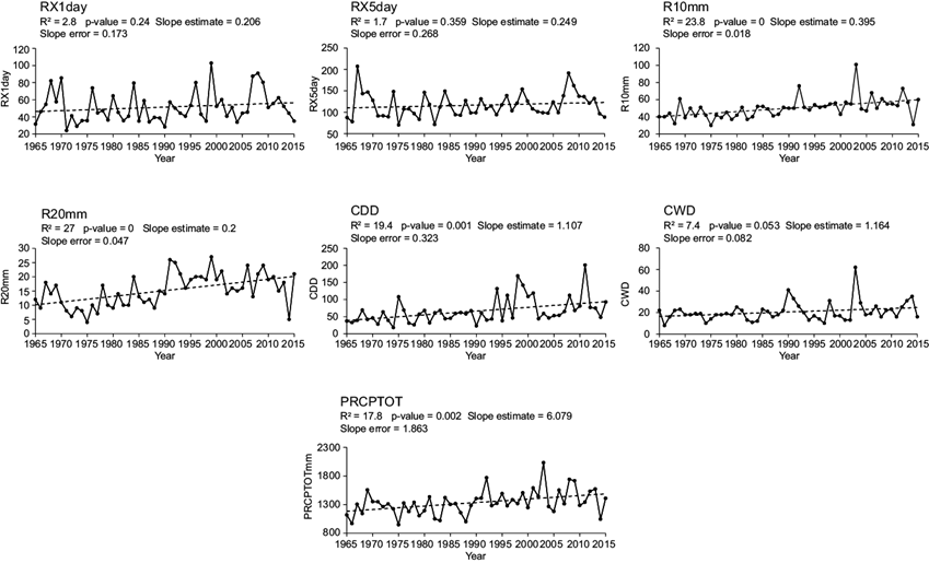
Figures 3 and 4 show the calculated temperature and precipitation indices. The graphs display the trend of each indicator (dashed line); the value of the slope and the p-value, as well as its R2 values are also indicated.
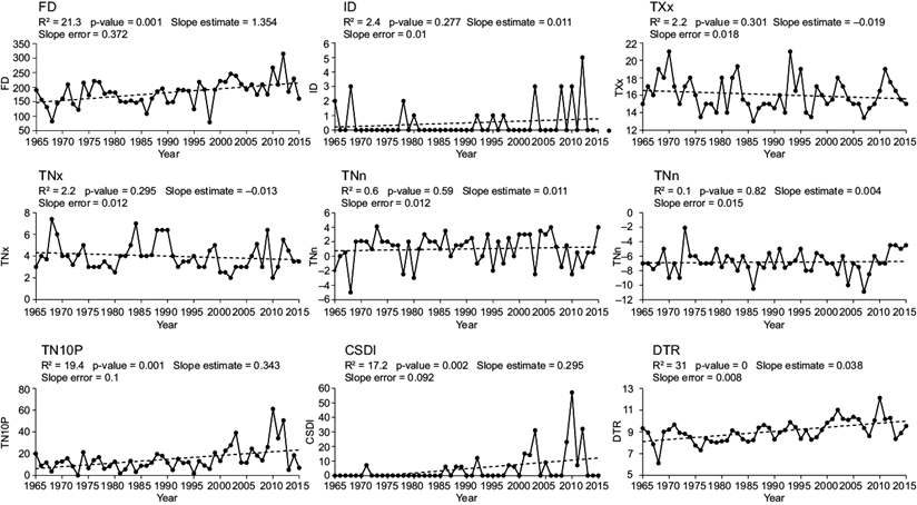
Note that only seven of the nine temperature indices have positive trends, but only four have significant positive trend. These are DTR, CSDI, FD and TN10p (p-value = 0, 0.002, and 0.001 for the last two, all respectively), in all cases with a level of significance of 0.05. The number of frost days (FD) tends to increase 1.3 days/year from 1965 to 2015; the icing days (ID) are very few per year, with only a couple of them on average. Its trend is far from significant and has a p-value of 0.277. The TXx index does not significantly change over time, which is confirmed by its p-value of 0.301. TNx has a non-significant decreasing trend (p = 0.295) while TXn has an even less significant increasing trend (p = 0.59). TNn has no significant tendency; its slope is 0.004 days/year and the p-value 0.82. The TN10p index shows a slightly positive trend, and the variation of 0.3 days/year turns out to be statistically significant. The duration of the cold periods (CSDI) that have been practically nonexistent at first, have increased considerably since the middle of the series; this is confirmed by a p-value of 0.002. Finally, DTR shows a significant positive trend; its increase of 0.04 days/year is associated with a p-value of zero.
All precipitation indices have an apparently positive trend, but only four of the trends are statistically significant. In order of appearance in Figure 4, even though the maximum precipitation in 1 day (R×1day) increases by 0.2 mm/year, it turns out to be statistically insignificant; its p-value is 0.24, but the required level of significance is α = 0.05. Likewise, the maximum precipitation over 5 days (R×5day) has no significant variation (p = 0.359). The R10mm index shows a tendency to increase by 0.4 days/year; its p-value of zero indicates a high level of significance. Similarly, although with less variation with time (0.2 days/year), days with precipitation of more than 20 mm (R20mm) have a positive trend justified by p = 0. The number of consecutive dry days (CDD) shows an increase equal to 1.1 days/year; the result is statistically significant with p = 0.001. The increase in the number of consecutive wet days (CWD) is not significant (p = 0.053). Finally, the total annual precipitation (PRCPTOT)increases 6.1 mm/year; this increase and its level of significance (p = 0.002) are clearly visible. Table I summarizes the above.
Table I Behavior of the indices over time.
| Variable | No. of ETCCDI | Index | Unit of measurement | P-value and significance1 (α = 0.05) Y/N | Change and trend2 +/- |
| Temperature | 1 | FD | Days/year | 0.001 Y | +1.354 |
| 3 | ID | Days/year | 0.277 N | +0.11 | |
| 6 | TXx | ºC | 0.301 N | +0.019 | |
| 7 | TNx | ºC | 0.295 N | -0.013 | |
| 8 | TXn | ºC | 0.59 N | +0.011 | |
| 9 | TNn | ºC | 0.82 N | 0.004 | |
| 10 | TN10p | Days/year | 0.001 Y | +0.343 | |
| 15 | CSDI | Days/year | 0.002 Y | +0.295 | |
| 16 | DTR | ºC | 0.0 Y | +0.038 | |
| Precipitation | 17 | RX1day | mm/year | 0.24 N | +0.206 |
| 18 | RX5day | mm/year | 0.359 N | +0.249 | |
| 20 | R10mm | Days/year | 0.0 Y | +0.395 | |
| 21 | R20mm | Days/year | 0.0 Y | +0.2 | |
| 23 | CDD | Days/year | 0.001 Y | +1.107 | |
| 24 | CWD | Days/year | 0.053 N | +0.164 | |
| 27 | PRCPTOT | mm/year | 0.002 Y | +6.079 |
1Significance: Y = yes, N = no; 2Trend: + = positive, - = negative.
There is a significant increase in the presence of FD at a rate of 1.3 days/year, but the number of days with maximum temperature below the freezing point (ID) remains almost constant with a trend of 0.01 days/year. The monthly highest maximum temperature and the monthly lowest maximum show an apparent decreasing tendency, while those of the monthly highest minimum temperature appears to remain constant. Although the trends in TXx and TNx are not statistically significant individually, together they generate a statistically significant increase in the diurnal thermal oscillation (DTR) over time with a value of +0.04 ºC/year. There is a significant increase in the percentage of cold nights (TN10p) as well as in the duration of the cold periods (CSDI). Both increase by 0.3 days/year.
The number of days with precipitation greater than 10 and 20 mm is increasing by 0.4 and 0.2 days/year, respectively; simultaneously, the consecutive dry days (CDD) increase by 1.1 per year. In contrast, there is no significant increase in maximum rainfall for periods of 1 and 5 days. The total annual rainfall clearly shows an increasing trend of 6.1 mm/year. Overall, all of the above suggest that precipitation occurs as increasingly isolated events, more concentrated and intense rainfall.
Figure 5 shows the average annual air temperature. Sen’s slope (Dawood, 2017; Kumar et al., 2017; Zeleňáková et al., 2018) is -0.0004 ºC/year, and the Mann-Kendall test indicates that it is not statistically significant (p value = 0.93). Hence, there is no sign of high mountain heating at the Nevado de Toluca station over the last 50 years, in terms of average temperature.
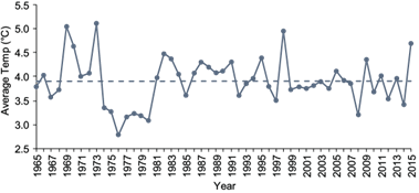
In comparison, Malamud et al. (2011) have analyzed temperature trends at the Mauna Loa Observatory (MLO, 3397 masl, 19.54 ºN) in Hawaii. The mean annual air temperature increased by 0.021 ºC/year from 1977 to 2006. This change is due to an increase in nighttime temperatures and associated with a decrease in the diurnal temperature range (DTR) by 0.050 ºC/year. A similar value for the mean annual temperature (0.019 ºC/year) was found by McKenzie et al. (2019) for the period 1955-2016. Hence, the air temperature trends in this island environment are markedly different from those on Nevado de Toluca.
Based on the time series of Figure 5, the short cooling period experienced in different parts of the planet during the 1970s (Chylek et al., 2009) can be clearly seen at the Nevado de Toluca volcano. This episode of thermal decline favored the small advances of the Mexican glacier cover (Cortés-Ramos et al., 2019).
The values of average temperatures and precipitation obtained for the last 30 years (1986-2015) (provisional climatic normal) are 8.7 ºC for the maximum annual temperature, -0.78 ºC for the minimum annual temperature and 4.0 ºC for the annual average. Annual Total precipitation is 1398.8 mm. Figure 6 shows graphically these values distributed among the months of the year.
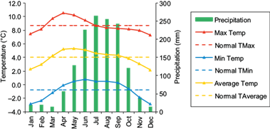
Fig. 6 Average monthly temperature and precipitation during the period 1986-2015 at the Nevado de Toluca weather station. Dashed lines represent the provisional normals for temperature variables.
Finally, no evidence was found for the influence of positive and negative ENSO events in site precipitation. Figure 7 shows the annual rainfall and ENSO periods from 1965 to 2015.
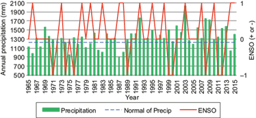
It seems that the only positive ENSO period that coincides with the year of maximum accumulated rainfall is 2003 and probably 1992, while the rest of the ENSO periods show no correlation. On the other hand, during the negative phases the coincidence is even minor, since even during the neutral phases of ENSO, the annual rainfall is lower than that recorded during the negative phases. To confirm the above, Figure 8 shows the 12 quarters with moving average that determine the ONI.
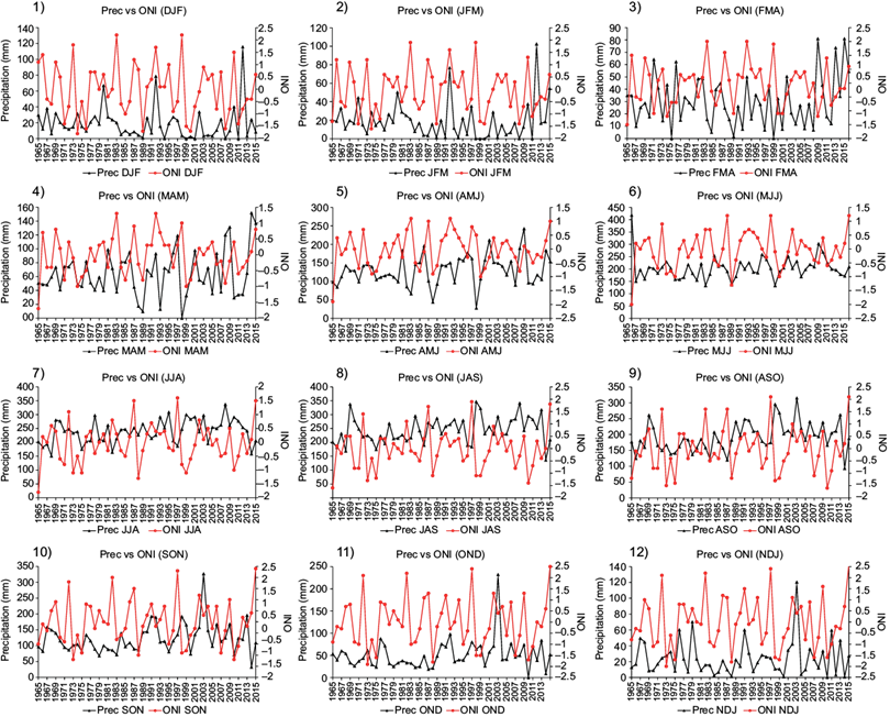
Fig. 8 Oceanic surface temperature anomaly observed in the ENSO 3.4 region (ONI) vs. the precipitation index in the Nevado de Toluca station. The initials in parentheses correspond to the first letter of the month in each of the quarters.
The sequence of graphs (1 to 12) demonstrates that the periods of ENSO (+ or -) do not directly affect the amount of precipitation in its corresponding period. Magaña et al. (1998) and Bravo-Cabrera et al. (2017) point out that during the rainy seasons, ENSO periods have no influence on the accumulated precipitation in the center of the country, emphasizing the above. Although these authors state that the opposite is true in drought periods, no type of correspondence was found with the accumulated rain in the Nevado de Toluca. Redmond and Tharp (1993)) state that the influence of the ENSO depends strictly on the characteristics of the relief and its distance to the ocean, therefore its influence varies throughout the national territory. In case of occurrence at this site, an increase in the pluvial rate could be noticeable at lower elevations and not in high mountain systems.
The rain regime that is recorded in the Nevado de Toluca weather station, which in itself is high compared to the records of the Morrena and Sierra Negra stations, could be a product of the heat islands that occur in the metropolitan area of Toluca city, as pointed out by Morales-Méndez et al. (2007). All of the above suggests that in the Nevado de Toluca, near the summit, the combination of negative trends in temperatures and positive trend of precipitation favors increasingly sporadic snowpacks during the winter, but that last more days.
5. Conclusions
We analyzed a half-century long time series from the Nevado de Toluca weather station (1965-2015). There is no significant trend in the annual average air temperature at the Nevado de Toluca volcano station, neither warming nor cooling over the last 50 years. However, there is an increase in the number of frost days, the duration of cold periods, and in the amplitude of the daily thermal oscillation. Total annual precipitation increases over time, although precipitation is increasingly concentrated. The combination of the above favors the permanence of seasonal snowpack although its appearance is increasingly sporadic. ENSO phases (+ or -) do not directly influence the rainfall rate in this high mountain.
High-mountain ecosystem studies can be considered later with the contribution of this work. Due to the scarcity of high-elevation climatic time series within the intertropical region of the planet, the results of this research may serve as a reference for climate variability in high mountain ecosystems. Examples of the above are the mountains of the northern Andes, the Kilimanjaro and the Hawaiian volcanoes. In the meantime, it is imperative to continue with uninterrupted data collection at this station, correct maintenance, and adequate documentation of the actions that are applied to the equipment in order to achieve a better quality of the data that will be recorded by this weather station in the future.

