


 nueva página del texto (beta)
 Inglés (pdf)
 Artículo en XML
 Referencias del artículo
 Enviar artículo por email
 Citado por SciELO
  Similares en
SciELO
Similares en
SciELO 
 Permalink
1. Introduction
When studying air quality, numerical models are useful for understanding the formation of aerosols and their evolution in the middle and lower atmosphere. The potential effects of aerosols significantly affect crops, natural ecosystems, water sources in snow-capped mountains and sky opacity, as well as the radiative forcing of the Earth (Seinfeld and Pandis, 2012). Furthermore, studying aerosols released from biomass burning is crucial because approximately 90% of biomass burning is caused by human activities (NASA, 2001).
In Peru, the cutting and burning of forests pose natural and anthropogenic threats, causing a loss of approximately 113 thousand hectares of forests per year (GGGI/DIE/SERFOR, 2015). Further, forests are mainly lost due to migratory agriculture and informal mining. The former is caused by the formation of abandoned areas once crops have exhausted the soil fertility, and the latter by indiscriminate felling of trees associated with ore exploration and gold mining activities. Aerosols are usually found in the atmosphere as solid or liquid particles; their aerodynamic radii vary between 0.001 and 100 µm. Such aerosols are generated by both natural and anthropogenic sources; they modify the radiative balance of the Earth in two ways: directly while interacting with the incoming solar radiations and outgoing terrestrial radiations (by dispersion and absorption of radiation) and indirectly through the modification of the microphysical cloud properties and precipitation processes (acting as condensation nuclei in the formation of clouds or modifying their optical properties and lifetime).
During biomass burning, emissions generated include multiple gaseous compounds and particles (Gao et al., 2003), which significantly impact tropospheric balances at all scales, i.e., local, regional, and global. Aerosols found in the atmosphere have an important characteristic: their size distribution, which identifies the number of aerosols present in a certain size range. Therefore, optical aerosol properties can be derived from the theory of dispersion (Toledano et al., 2007). The phenomenon of dispersion takes into account the relationship between the radius of the particle and the wavelength of the incident radiation. In the event that the radius of the particle exceeds or approaches the incident wavelength, the probability of dispersion of the radiation in the direction of the beam increases and the backscatter decreases, which is called the phase function and allows us to characterize aerosols when the size of their particles are diverse compared to the wavelength of the radiation that affects them (Sumalave, 2015). Summing-up, the dispersion itself involves a physical process in which a particle extracts energy from incident radiation during its trajectory and radiates this energy in all directions, which is a critical concept for this study.
Atmospheric aerosols are known to affect both air quality and climate change (Kaufman et al., 2002; IPCC, 2007). In terms of air quality, high-surface-level aerosol concentrations are strongly associated with impaired visibility (Baumer et al., 2008) and adverse effects on human health, such as respiratory and cardiovascular diseases (Pope III et al., 2002; Kappos et al., 2004; Brook et al., 2010; Brauer et al., 2012).
The relationship between PM10 and aerosol optical depth (AOD) depends on many factors and is affected by various parameters. There is a so-called direct effect whereby aerosol particles disperse incoming sunlight (short wave) back into space, which affects the overall radiation balance and influences AOD. There is also an indirect effect, which is related to the property of aerosols acting as cloud condensation nucleus (CCN). So its variability affects the number, density, and size of cloud drops. This can change the quantity and optical properties of clouds, and therefore their reflection and absorption (Tao et al., 2012).
For the same study area and data set , this correlation could significantly change throughout the year due to the variable source and meteorological changes. Empirical studies of the relationship between PM2.5 and AOD have been reported in various regions of the world (Gupta et al., 2006; Ho and Christopher, 2009; Kusmierczyk-Michulec, 2011), such as the US (Wang and Christopher, 2003; Zhang et al., 2009), the densely populated and industrially developed areas of Asia (Kumar et al., 2007; Mukai et al., 2007), and Europe (Kacenelenbogen et al., 2006; Schaap et al., 2009; Pelletier et al., 2007; Dinoi et al., 2010). Nevertheless, as noted in the work of Schaap et al. (2009), locally obtained relationships between AOD and particle matter (PM) cannot be easily extrapolated to other areas owing to variations in different source types, PM composition, and meteorology. Variations in local meteorological conditions, multiple aerosol layers, and changes in chemical aerosol composition likely play an important role in determining the strengths of such relations. Therefore, continued research is needed to quantify PM-AOD relationships in various regions of the world, being the main reason that aerosols (in particular PM) have a great influence on incident and outgoing radiation, generating the so-called greenhouse effect. On the other hand, in many countries like Peru, there are no monitoring networks that measure PM levels and few surface measurements have been obtained to date, so it is impossible to quantify them directly to assess their impact on the climate. Therefore, if we know the PM-AOD relationship, we can estimate its scope and effect. Koelemeijer et al. (2006) demonstrated that the correlation between PM and AOD improved when AOD is divided by the mixing layer height, and, to a lesser extent, when it correlates aerosol growth with relative humidity. Thus, the relationship between AOD and PM should be determined regionally. Kong et al. (2016) showed that the correlation between PM2.5 and PM10, and AOD from the Moderate Resolution Imaging Spectroradiometer (MODIS) onboard the Terra and Aqua satellites, was similar to the correlation between PM2.5 and PM10 concentrations, and the AOD observed on the ground. Studies conducted in Asia state that when empirical models are used to evaluate hourly PM10 estimations using AERONET and MODIS datasets, improved performances are observed (Seo et al., 2015).
In most parts of the world, excluding South America, considerable research has been conducted using the Weather Research and Forecasting model coupled with chemistry (WRF-Chem) to study biomass burning. For example, in the eastern Mediterranean (Aegean Sea), a study used this model to discuss the influence of biomass burning during summer (Bossioli et al., 2016). This study assessed chemical variables, such as ozone (O3) and particulate matter with a diameter of 2.5 μm or less (PM2.5) together with meteorological variables, such as temperature and wind, among others, for the period between August and September 2011. The study concluded that biomass burning significantly increased O3 and PM2.5 concentrations. In China, an important biomass and fossil fuel burning study was conducted by Ding et al., (2013), whose results showed the effects of the combination of different atmospheric pollutants (such as aerosols) on air temperature and rainfall. Moreover, agricultural burning and fossil fuel pollution can reduce solar radiation by more than 70%, sensible heat by more than 85%, and air temperature by approximately 10 K, in addition to significant impacts on rainfall during the day and night cycles. Xu et al. (2018) also studied the effects of biomass burning on black coal in South Asia and the Tibetan Plateau using the WRF-Chem model. In that study, the lowest and highest concentrations were recorded during winter and spring, respectively, just along the foothills of the Himalayas. Finally, the research suggested that the emissions released by biomass burning significantly affect the deposition of black coal on glaciers in the Tibetan plateau, which may thaw glacier snow and cause significant environmental problems owing to the pollution of water resources.
In the particular case of Peru, the dispersion and transportation of PM10 produced by biomass burning in Peru and its neighboring countries was studied with data of 2015 (Moya et al., 2017). In that work, it was concluded that the presence of PM10 in Peru is a consequence of the burning of vegetation in the country itself, but also in neighboring countries. A good correlation was also found between AOD and PM10; however, only June, July and August were taken into account, without considering September, when traditionally burning takes place in the country, so that this work can be considered as preliminary. In this study, we considered the months of 2017 in which, both historically and traditionally, biomass burning is more significant, which includes the entire June-October period. The fact of having carried out the study for another year also serves as a complement to the previous work. In addition, this study contemplates the rigorous analyzes of meteorological variables observed during the study period. It is the only work that relates PM10 to AOD in the region.
This research article is organized as follows: section 2 describes the domain, main model configurations, and data used; section 3 presents the simulation results and compares them with the observed data, and finally section 4 outlines the conclusions of the research.
2. Data and methodology
2.1 Study area
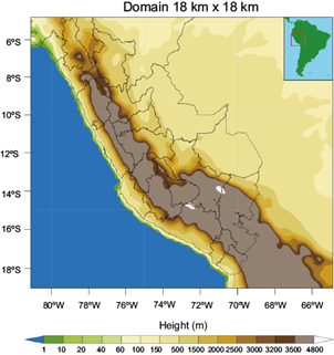
The central Peruvian Andes are located between 8º-17º S and 68º-80º W, as shown in Fig. 1, and comprise three mountain ranges: the Central Range, which is discontinuous owing to transversal erosion by the Apurímac and Mantaro rivers, where a part of the Mantaro basin is also located; the Western Range, which is the highest range serving as a watershed between the slopes of the Pacific Ocean and the Amazon River; and the Eastern Range, which is a low and discontinuous range extending through the high jungles of the Cusco and Junín departments. These mountain ranges are crucial as they determine and/or modify the regional climatic conditions and include the main reserves of drinking water, thus affecting local agriculture and the economy.
2.2 Model description
We used the WRF-Chem model version 3.7 with a single 18 km domain covering nearly the entire Peruvian territory, as shown in Figure 1. In the perpendicular plane, the model has been configured with 32 vertical levels for five simulation months, from June to October 2017. The period was extended to include June as a buffer. Table I lists the main parametric configurations used in the model to represent physical and chemical processes, and Table II lists the main configurations for the preprocessing phase. The physical and chemical schemes were selected based on the results obtained from previous research studies (Hu et al., 2010; Grell et al., 2011; Álvarez et al., 2017; Moya-Álvarez et al. 2018a, b, 2019).
Table I Physical and chemical parameterizations.
| Chemistry and atmospheric process | Scheme |
| Long-wave radiation | RRTMG |
| Short-wave radiation | RRTMG |
| Surface layer | Monin-Obukhov |
| Earth surface | Noah |
| Planetary boundary layer | ACM2 |
| Cumulus | Grell-Freitas |
| Microphysics | Lin (Purdue) |
| Gas phase chemistry | RADM2 |
| Aerosol module | MADE-SORGAM |
| Photolysis | Fast-J |
Table II Domain and boundary conditions used.
| Grid size | 18 km |
| Domain center | (-12.0, -73.5) |
| Number of points in x | 90 |
| Number of points in y | 100 |
| Number of points in z | 32 |
| Boundary condition frequency | 6 h |
| Meteorological fields | FNL 1 × 1 |
| Time step | 90 s |
| Simulation period | 5 months |
The Rapid Radiative Transfer Model for General Circulation (RRTMG) was used to assess short- and long-wave radiations and heating rates. RRTMG is a validated and correlated k-distribution band model used for calculating long-wave flows and heating rates (Price et al., 2014). The Monin-Obukhov surface layer scheme, which uses the theory of similarity to establish a relationship between diffusion coefficients and turbulent kinetic energy, was also used (Hill, 1989). For the planetary boundary layer, the Asymmetric Convective Model version 2 (ACM2) was used (Pleim, 2007). This model includes a first-order eddy diffusion component in conjunction with an explicit non-local transport of the original ACM scheme. This modification is designed to improve the shape of vertical profiles near the surface. To model the clouds, we used Grell-Freitas convection parameterization, wherein the mass flow of the cloud base quadratically varies as a function of the convective updraft fraction in the global non-hydrostatic model (Fowler et al., 2016). Then, for microphysics, we used the Purdue-Lin scheme, which is relatively sophisticated in the WRF model. This scheme includes six hydrometer classes: water vapor, cloud water, rain, cloud ice, snow, and graupel: it is suitable for mass-parallel calculations, as there are no interactions between the points in the horizontal grid (Mielikainen et al., 2016). From the perspective of the chemical variables, the Regional Acid Deposition Model version 2 (RADM2) was used for gasses (Chang et al., 1989). The inorganic species included in the RADM2 mechanism are 14 stable intermediates, four reactive intermediates, and three abundant stable species, such as oxygen, nitrogen, and water. The aerosol module used herein is based on the Modal Aerosol Dynamics Model for Europe (MADE) (Ackermann et al., 1998), which incorporates the Secondary Organic Aerosols Model (SORGAM), jointly referred to as MADE-SORGAM, together with aerosol dynamics, such as nucleation, condensation, and coagulation. MADE-SORGAM considers the classical modal description of the atmospheric aerosol diametric distribution through three continuous log-normal distributions, which are Aitken, accumulation, and coarse modes, approximately corresponding to the PM10-PM2:5 range. Finally, photolysis frequencies are calculated using the Fast-J scheme, which calculates the photolysis rate in the presence of an arbitrary mixture of cloud and aerosol layers. The algorithm is fast enough to allow the scheme to be incorporated into the 3-D global chemical transport models with photolysis rates updated every hour (Wild et al., 2000).
In the WRF-Chem model configuration, the initial condition for aerosol PM10 is its total absence in the chosen domain. Moreover, the model maintains by default and during its simulation process the amount of PM10 pollutant constant at the domain limit.
2.3 Data
This study uses three different types of data. The first one is the meteorological FNL (final) Operational Global Analysis data (UCAR-NCAR, 2015) (altitude and wind, among others) obtained from the National Center of Environmental Prediction (NCEP), which serve as initial and boundary conditions for the WRF model and are presented in 1º × 1º grids prepared operationally every 6 h. FNL data are obtained using the same model that NCEP uses in the global forecast system (GFS); however, they are prepared approximately 1 h after the GFS is initialized to obtain more observation data. These data are freely accessible and can be downloaded from the following website: https://rda.ucar.edu/datasets/ds083.3/index.html?hash=sfol-wl-/data/ds083.2&g=22017. Available since 2015, these data contain around 72 parameters, from which the following variables may be highlighted: pressure at sea level, geopotential altitude, air temperature, regional, meridional and vertical wind components, and surface temperature of the sea and soil parameters.
It is important to notice that these latest data derive from the numerical predictions of the Global Forcast System (GFS) model and they are the ones that feed the UCAR-NCAR FNL, so they lead to errors that have an impact on the imprecision of the final forecast.
The second set of data was obtained from the NCAR Fire Inventory (FINN), which includes emissions calculated in near real-time based on fire numbers with information obtained from MODIS. All data files contain the global daily fire emission estimates with an approximate resolution of 1 km2 and multiple chemical variables, but only PM10 was used for our purposes. The download link for these data is https://www.acom.ucar.edu/acresp/dc3/finn-data.shtml.
Finally, the third data type corresponds to AOD at a wavelength of 440 nm registered at the Huancayo observatory by the CIMEL photometer. We recovered the data used by AOD from the AERONET monitoring network belonging to NASA, in which the standardization, calibration and processing processes are carried out. Both experimental AOD measurements and simulated outputs were divided by their respective average values, which allowed us to compare their values.
Topography has also been considered in the model. Data from the Global 30 Arc-Second Elevation (GTOPO30) of the United States Geological Survey (USGS), which are a default option in the model, were replaced by the digital elevation model of the Shuttle Radar Topography Mission (SRTM; https: //dds.cr.usgs.gov/srtm/version2_1/) (Rodríguez et al., 2006; Farr et al., 2007), which improves the continental digital elevation model GTOPO30 (Gesch et al., 1999) approximately 10 times (both in spatial resolution and vertical accuracy). However, for South America, it has errors that exceed 100 m.
3. Results
Figure 2 shows the average number of forest fires observed by the satellite over the simulation domain. Here, the number of fires increased in July (451), August (1006), and September (1474) and decreased in October (947). The total fire distribution for these four months is shown in Figure 3.
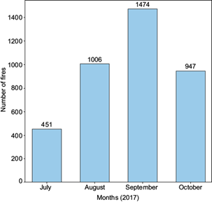
Fig. 2 Monthly average number of fire outbreaks observed by MODIS onboard the Terra and Aqua satellites during the studied period.
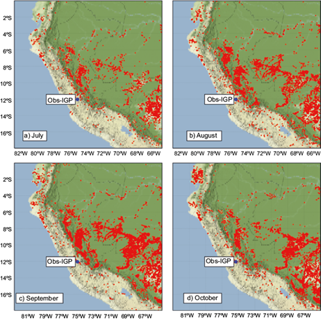
Fig. 3 Forest fire distribution for the 4-month study period. Red dots denote the fires registered by the satellite. The location of the sun photometer is marked with a blue dot.
As can be seen, even when there have been fire outbreaks in Peru, Ecuador, Colombia, Brazil, and Bolivia, the largest number of fire outbreaks in the studied regions occurs in Brazil and Peru. In the latter, the greatest number of fires is observed within the Peruvian high jungle.
From Figure 4 it can be observed that AOD increases from July to August in correspondence with the number of fires. This trend is observed between the second half of September and October. In contrast, during the second half of August and the first half of September, this relationship weakens as fire outbreaks in this period occurred in areas far from the observatory of Huancayo and did not influence AOD at the observation point. The correlation obtained between AOD and the number of recorded fire outbreaks was 0.77, which indicates a strong linear relationship. Therefore, we can say that the volume of vegetation burning significantly influences AOD in the city of Huancayo. In the same figure a time lag can be observed between AOD measurement and the number of recorded fire outbreaks owing to the distance between the photometer and the fire outbreaks. Therefore, it is important to consider the meteorological conditions (wind direction and speed) in this study.
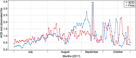
Fig. 4 Normalized curves of the number of fires recorded by the satellite and AOD, as denoted by the blue and red lines, recorded at the Huancayo observatory.
Figure 5 shows monthly average PM10 concentration levels obtained using the model at the Huancayo observatory. According to the number of fires in Figure 2, the highest concentration levels occurred in August and September.
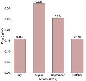
Figure 6 shows the PM10 concentrations for each of the months studied, as predicted by the model for the study area. As can be seen, the highest concentrations correspond to areas where the largest number of fire events is reported. The highest PM10 value is approximately 10 µg m-3, and the maximum area covered by this pollutant corresponded to September. In July, the PM10 concentration value reached an average of up to 3.5 µg m-3, with some PM10 concentration values exceeding 10 µg m-3. In August, PM10 values increased with concentrations exceeding 10 µg m-3, achieving the highest value in September but decreasing in October.
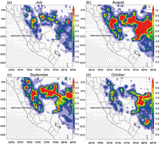
Fig. 6 PM10 (µg m-3) distribution in the study area during the four months of evaluation. These data correspond to the simulations performed by the model. The black dot represents the location of the sun photometer.
In Peru, the largest areas with PM10 concentrations exceeding 10 µg m-3 are observed during August and September in the high jungle area. In the department of Junín, the highest values, ranging between 2.5 and 10 µg m-3, were recorded in August and September in the Mantaro basin and jungle areas, respectively.
At the Huancayo observatory, PM10 values obtained using the model correspond to a large extent with the total number of fires, as can be seen in Figure 7. A Pearson’s r of 0.65 indicates a moderate positive linear relationship between PM10 and the fire outbreaks. In Figure 7 it can be observed that when the number of recorded fire outbreaks increases, the PM10 concentration also increases. Similarly, low PM10 values correspond to a decrease in the number of fire outbreaks, as reported in the middle of August and September.
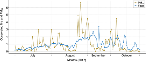
Fig. 7 Normalized curves comparing the number of fires observed (blue line) and PM10 predicted by the model (light green line) for the study period.
Figure 8 shows the relation between PM10 and AOD recorded at the Huancayo observatory. The Pearson’s r between those two magnitudes was 0.57. In this case, PM10 increases during August, which corresponds to a gradual increase in AOD, which in turn reaches its maximum value in the first 10 days of August and decreases in the middle of the month. The same phenomenon occurs with PM10 concentrations and the number of fire outbreaks recorded in Figure 7. During the first half of September, AOD does not follow the same concentration-increasing trend; however, in the first half of October, both PM10 concentrations and AOD increased and decreased towards the middle of the month. The relationship found between the burning of biomass and AOD ratifies the physical processes that take place between particles suspended in the atmosphere and radiation, according to the theory of dispersion, addressed in the works of Toledano et al. (2007).
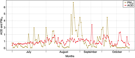
Fig. 8 Normalized curves comparing the AOD (red line) and PM10 (light green line) predicted by the model during the study period.
Although all correlations of the studied variables exceed 50%, better correspondence exists between AOD and the number of fire outbreaks observed in the domain area. A possible explanation could be that the inaccuracies in the forecast are associated with the model’s failure in generating air circulation patterns, which may be related to the complex orography of the place. Another important aspect is that only the influence of PM10 on AOD is investigated in this work, whereas the burning of vegetation implies the release into the atmosphere of many other elements that can influence AOD. Notably, the axis of the plumes is neither close to nor passes over the measurement point; thus, the values recorded by the sun photometer could show a time lag between the AOD values and the fire sources.
4. Circulation patterns
At the surface level (few meters above the ground) wind shows a chaotic behavior due to local topography (valley and mountain winds); even pollutants are also transported to higher levels in the atmosphere. Because of that, we considered the vertical average of wind speed and direction up to 1500 m (Fig. 9) from July to October. In July and September, we observed that winds are directed in an east-west direction and from south to north. On the other hand, in the region of the Peruvian coast and for August and October the predominance of the wind continued from south to north; however, in the Amazon region the wind direction had a pattern that went from north to south. In the Mantaro valley region, where the Huancayo observatory is located, the wind speed ranged between 4-8 m s-1. Throughout the study period, there was a notable decrease in wind intensity throughout the Amazon/Andes transition zone, due to the effect that causes the presence of the Andes mountain range, as well as the convergence of these winds over the entire mountain range.
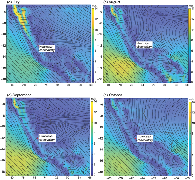
Fig. 9 Arrows represent the vertical average of all the levels considered in the monthly wind speed and direction model. The scale of colors indicates the wind speed in m s-1 for each map. The red dot indicates the location of the Huancayo observatory.
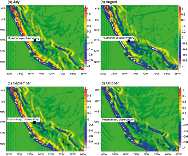
4.1. Vertical movements
Figure 10 shows the monthly vertical movement averages obtained from the simulation in WRF-Chem over the study area for the July-October period. The Huancayo observatory is located on the Mantaro valley, where there is a predominance of winds with ascending movements, which explains the low concentration levels of PM10 thrown by the model. Descending winds, which increase from July to October, prevail over the transition zone from the Amazon to the Andes, favoring aerosol concentrations over the lowest surface levels, as shown in Figure 6. Above the Andes mountain range, ascending movements may be observed, some exceeding -1 Pa s-1. These movements begin to decrease in July, continuing through October. As expected, the movements are generated by wind convection above the Andes, whereas, along the Peruvian coast, descending movements may be observed.
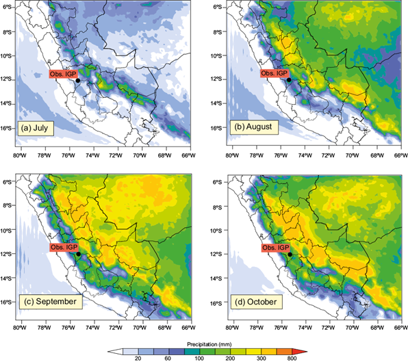
4.2. Monthly rainfall
As seen in Figure 11, rainfall increases from July to October, and the highest values are recorded along with the hotspot (Espinoza et al., 2015). The maximum precipitation occurs in October, with values exceeding 480 mm in the study area. Therefore, the annual rainfall increase recorded in October is an important factor for the decrease of fires in a large part of the Peruvian territory. As can be seen, the behavior of the low concentrations of PM10 and the decrease in the number of fire foci during the analyzed period corresponds to the rainfall regime. Besides, Figure 8 shows how PM10 levels also decrease during October, validating-as expected- an inverse relationship between rainfall and pollutants.
5. Conclusions
In this work, we studied the influence on AOD of PM10 particles produced by the burning of biomass, as measured at the Huancayo observatory in the Mantaro basin. To this end, the WRF-Chem model was used configured with an 18-km resolution domain. FNL data were used as input meteorological data, and FINN data were used as emission data to feed the model. The fire inventory assessed the number of fire outbreaks recorded by the satellite during the four-month study period, indicating an increase in fire outbreaks from July to September 2017, and a slight decrease during October 2017. Between August and September, in which the weather conditions favor biomass burning, the anthropogenic factor must be considered, since fire events are initiated during this period to prepare the soil for planting during the upcoming monsoon. We obtained a good correspondence between the temporal distribution of the number of fire outbreaks reported during the study period and AOD, thus demonstrating the influence of biomass burning on AOD in the study region.
In correspondence with the number of fire outbreaks, PM10 concentrations increased from July to September and decreased in October. The highest concentration values were recorded during the early morning when atmospheric stability is high. Consequently, higher subsidence was recorded at times when the wind speed was low. In general, the highest obtained PM10 concentration values were around 10 µg m-3 in the lower Mantaro basin.
The rainfall generated by the model showed a continuous increase between July and October. An increase in the rains during October contributed to the decrease in the number of fire outbreaks and PM10 concentrations owing to the wet deposition or particle washing process.
The PM10 values generated by the model showed the same tendency as AOD, but with less correspondence, which can be attributed to model inaccuracies.
Based on the analysis of fire outbreaks, PM10 concentrations, and AOD, this study has successfully demonstrated the impact between biomass burning and AOD for the first time in Peru. This relationship found in general between the burning of biomass and AOD ratifies the physical processes that take place between suspended particles in the atmosphere and radiation.
With reference to the previous study conducted for Peru, in this work the relationship between biomass burning and AOD was ratified, mainly based on the results obtained from its comparison with the number of outbreaks. In this regard, it should be noted that in the present investigation, the correlation between PM10 obtained with the model and the AOD was not as effective as in the previous work.

