


 text new page (beta)
 English (pdf)
 Article in xml format
 Article references
 Send this article by e-mail
 Cited by SciELO
  Similars in
SciELO
Similars in
SciELO 
 Permalink
1. Introduction
Climate variability has direct and indirect impacts on natural and human systems. Spatial and temporal rainfall variability leads to an increased incidence of extreme events, such as floods and droughts, with direct effects on the economy, agriculture, urban structure and human health.
In regions with transitional climates, such as areas of contact between the tropics and subtropics, climate variability has been shown to be extremely dynamic, and, thus, its impacts have become more notable, resulting in conditions of lesser predictability (Sant’Anna Neto, 1999). This complexity combined with disturbances of tropical (low latitudes) and extratropical (high latitudes) atmospheric systems, where rainfall is the main element of climate variability, is also observed in the climatic dynamics of Paraná State, located in southern Brazil.
Rainfall variability in Paraná State has been historically discussed and studied in a systematic way, with classic works like those of Monteiro (1968), Nimer (1979) and Maack (1981), who developed the first studies about rainfall genesis and its spatial-temporal distribution based on a few precipitation stations. Surface meteorological networks of observed data with longer time series (more than 30 years) have only been available within the last decade in Brazil; as a consequence, it is only now possible in Paraná State to identify areas and periods that have experienced decreases and increases in rainfall.
In this context, an important number of studies about rainfall variability in Paraná State have been developed, using a larger network of stations and employing more robust and sophisticated analysis. Several studies have offered more plausible explanations of rainfall variability and impacts, e.g., the works of Nery et al. (1996, 1997), Silva and Guetter (2003), Grimm (2009a, b), Nascimento Jr. (2013), Carmello and Sant’Anna (2016), Nascimento Jr. and Sant’Anna (2016), Ely and Dubreuil (2017), Terassi and Galvani (2017) and Ely (2019).
Our interest in this paper is to present statistical parameters describing precipitation variability in Paraná State and to discuss the process of rainfall tropicalization, which refers to a set of trends that shows increased or concentrated precipitation with greater seasonality. Rainfall tropicalization can be understood as local and regional processes and impacts of climate change, which can be observed mainly by changes in the precipitation regime and the intensification of tropical climatic characteristics, e.g., the humidification of the rainy season or increased dryness during the dry season.
An important group of studies (Nascimento Jr., 2013; Carmello and Sant’Anna Neto, 2016; Nascimento Jr. and Sant’Anna, 2016; Ely and Dubreuil, 2017; Terassi and Galvani, 2017; Ely, 2019) has shown evidence that trends and changes in rainfall patterns in Paraná are mainly observed with the increase of rainfall during the humid period (which coincides with summer and spring), especially in the southern sector of the state.
However, the rainfall tropicalization process is not exclusive of Paraná State. It has been observed in other contexts and scales in tropical and subtropical regions that show an important increase in precipitation during the rainy season in tropical regions (Tomozeiu et al., 2000; Back, 2001; Blain et al., 2005; Marengo and Alves, 2005; Haylock et al., 2006; Salarijazi et al. 2012; Zarenistanak et al. 2014; Debortoli et al., 2015; Tozato et al., 2014; Hasan et al., 2014; Addisu et al., 2015).
Tomozeiu et al. (2000) used these tests and evaluated alterations in precipitation time series in the region of Emilia-Romagna, Italy, where much of the area shows a tendency towards increase, mainly after 1962. In India, tests were applied by Taxak et al. (2014), who observed that precipitation in the Waingangarante basin has declined -8.45% in recent years; positive trends were only observed in the post-monsoon period (March, April, and May).
In Bangladesh, Hasan et al. (2014) detected an increase in precipitation of 8.5 mm yr-1, which is more important during the rainy season and statistically significant in the pre-monsoon period (March, April, and May). There was a decrease in rainfall only in the dry season (December, January, and February). In Ethiopia, negative trends in precipitation between -3.947 and -1.561 mm yr-1 were observed by Addisu et al. (2015) in the sub-basin of Lake Tana; this was verified in for months except June, which presented a positive trend. In Iran, Salarijazi et al. (2012) and Zarenistanak et al. (2014) detected trends and a change point in annual hydroclimatic series of the Karun River and in annual and seasonal precipitation and temperature series of the southwest of the country. Yeh et al. (2015) elaborated spatial and temporal analyses of flooding in the northeast of Taiwan, and found monthly and seasonal precipitation averages of 72.2% during the the spring.
For South America, Haylock et al. (2006) observed increasing trends in total annual precipitation values in Ecuador, Paraguay, Uruguay, northern Peru, southern Brazil, and northern and central Argentina. Villar et al. (2009) studied the variability of the Amazon River in Peru using trends and change points tests, and observed rainfall decreases, with an estimated annual rate of -0.32%.
Back (2001), Blain et al. (2009), Marengo and Alves (2005), Debortoli et al. (2015), Tozato et al. (2014) and Tozato (2015) verified rainfall change points and trends in the states of Santa Catarina, Rio Grande do Norte, Paraíba, Ceará, Pernambuco, Bahia, and Amazonas. Debortoli et al. (2015) observed important precipitation alterations and trends in the southern Amazonia (about 45.0% of the region), mainly during spring and autumn.
This work adds to the set of studies about rainfall tropicalization impacts observed in Paraná State. Our specific objective is to present a spatial and temporal analysis obtained by applying the Mann-Kendall and linear regression tests, considering the period from 1976 to 2011. Statistical parameters are shown to indicate trends and the tropicalization process in the area.
2. Study area
Paraná State is located in southern Brazil, between 48º-52º W, 22º-25º S, with 199.315 km² of territorial area. Its climate varies from tropical, in the northern sector, to subtropical, in the central-southern sectors (Fig. 1).

In this context, due to its southern position in relation to Brazil, rainfall variability is basically determined by the occurrence of tropical and extratropical systems, specifically determined by the positioning and migration of the Atlantic Subtropical High, equatorial air mass intrusions from the Amazon, and polar frontal systems from the South Atlantic and their interactions with topography.
In general, precipitation is characterized by unimodal and bimodal patterns, which indicate configurations of the subtropical summer monsoon and a climatic transition area (Zhou and Lau, 1998; Grimm and Zilli, 2009; Marengo et al., 2012). In the northeast, the summer monsoon presents maximum precipitation in the trimesters form December to February, or from January to March; while in the west, the highest precipitation moves from summer to spring, beginning at the end of winter (Grimm and Zilli, 2009; Grimm, 2009a).
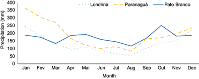
This climatic transition characteristic was also highlighted by Pereira et al. (2008), who observed the existence of greater differentiation between the dry and rainy seasons in the northern and western sectors, while in the southern sector, rainfall is uniformly distributed throughout the rainy season, marking seasonality in a rainy and a less rainy period.
This situation can be observed in the rainfall monthly averages of Londrina, Paranaguá, and Pato Branco on the northern coastal sector and in the southern sectors, respectively. The rainfall regimes of Paranaguá and Londrina show a classical pattern of tropical climate, while in Pato Branco, the annual variation does not show clear differences between rainy and dry season (Fig. 2).
Precipitation is produced by the synoptic systems formed in the South Atlantic Convergence Zone (ZCAS) (which has more influence in the north of the state, especially in extreme years), and extratropical, tropical, intertropical, and polar systems (Souza, 2006; Grimm, 2009a).
The influence of teleconnection patterns has been observed by Silva and Guetter (2003), Grimm et al. (2004), Souza (2006), Nascimento Jr. (2013) and Silva et al. (2015) in Paraná, where the Atlantic and Pacific Oceans demonstrate their influence through the El Niño Southern Oscillation (ENSO) interannual modes and moderate-to-weak decadal modes such as the Pacific Decadal Oscillation.
3. Data
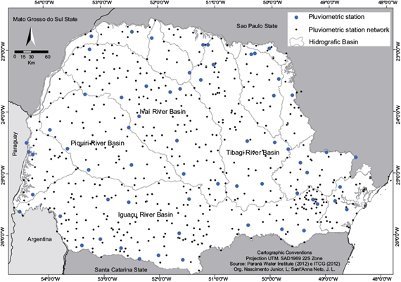
The data used in this study correspond to monthly rainfall (mm) in the historical series from 1976-2011 of 63 rainfall stations (Table I and large points in Fig. 3), from a total of 620 stations (small points in Fig. 3) available in the surface network, from the Paraná Water Institute.
Table I Pluviometric stations, county, geographic location, altitude, and percentage of missing data.
| Nº | Pluviometric station | County | Latitude | Longitude | Altitude | MD (%)* |
| 1 | Corrego Comprido | Corrego Comprido | 24º 45’ 00” | 48º 28’ 59” | 160 | 0.0 |
| 2 | Colonia Santa Cruz | Paranaguá | 25º 35’ 48” | 48º 37’ 29” | 32 | 7.0 |
| 3 | Colonia Cachoeira | Antonina | 25º 13’ 59” | 48º 45’ 00” | 80 | 0.0 |
| 4 | Morretes | Morretes | 25º 28’ 00” | 48º 49’ 59” | 8 | 0.0 |
| 5 | Capela Da Ribeira | Adrianópolis | 24º 40’ 48” | 49º 00’ 00” | 180 | 0.0 |
| 6 | Fazendinha | São José dos Pinhais | 25º 31’ 09” | 49º 08’ 48” | 910 | 0.0 |
| 7 | Curitiba | Curitiba | 25º 26’ 47” | 49º 13’ 51” | 929 | 2.0 |
| 8 | Costas | Rio Branco do Sul | 25º 00’ 37” | 49º 20’ 27” | 480 | 0.0 |
| 9 | Rio Da Várzea Dos Lima | Quitandinha | 25º 57’ 00” | 49º 22’ 59” | 810 | 0.0 |
| 10 | São Sebastião | Cerro Azul | 24º 51’ 00” | 49º 28’ 00” | 480 | 3.8 |
| 11 | Bateias | Campo Largo | 25º 21’ 00” | 49º 31’ 00” | 890 | 0.3 |
| 12 | Santana Do Itarare | Santana do Itararé | 23º 45’ 16” | 49º 37’ 21” | 543 | 0.0 |
| 13 | Tabor (Fazenda Marão) | Castro | 24º 37’ 59” | 49º 40’ 59” | 1100 | 0.0 |
| 14 | São Bento | Lapa | 25º 55’ 59” | 49º 46’ 59” | 750 | 0.0 |
| 15 | Est Criacao Estado | Joaquim Távora | 23º 30’ 00” | 49º 52’ 00” | 512 | 0.0 |
| 16 | Pirai Do Sul | Piraí do Sul | 24º 31’ 45” | 49º 55’ 44” | 1068 | 0.3 |
| 17 | Tomazina | Tomazina | 23º 46’ 00” | 49º 57’ 00” | 483 | 0.3 |
| 18 | Est. Experimental Cambará | Cambará | 23º 00’ 00” | 50º 01’ 59” | 450 | 3.5 |
| 19 | Santa Cruz | Ponta Grossa | 25º 12’ 00” | 50º 09’ 00” | 790 | 0.0 |
| 20 | Andirá | Andirá | 23º 04’ 59” | 50º 16’ 59” | 375 | 0.0 |
| 21 | Fac Agronomia Bandeirantes | Bandeirantes | 23º 06’ 00” | 50º 21’ 00” | 440 | 0.0 |
| 22 | São Mateus Do Sul | São Mateus do Sul | 25º 52’ 32” | 50º 23’ 22” | 760 | 1.0 |
| 23 | Tibagi | Tibagi | 24º 30’ 39” | 50º 24’ 40” | 720 | 0.0 |
| 24 | Imbituva | Imbituva | 25º 14’ 15” | 50º 36’ 02” | 869 | 0.5 |
| 25 | Tres Cantos (Despedida) | Leópolis | 22º 57’ 00” | 50º 37’ 59” | 904 | 0.3 |
| 26 | Rio Dos Patos | Prudentópolis | 25º 12’ 00” | 50º 55’ 59” | 690 | 0.0 |
| 27 | Faz.criacao Estado - Ibiporã | Ibiporã | 23º 16’ 00” | 51º 01’ 00” | 484 | 0.0 |
| 28 | Bela Vista Do Paraiso | Bela Vista do Paraíso | 22º 57’ 00” | 51º 12’ 00” | 600 | 0.0 |
| 29 | São Luiz | Londrina | 23º 31’ 00” | 51º 13’ 59” | 740 | 3.0 |
| 30 | Arapongas | Arapongas | 23º 24’ 00” | 51º 25’ 59” | 793 | 1.5 |
| 31 | Guarapuava | Guarapuava | 25º 27’ 00” | 51º 27’ 00” | 950 | 0.0 |
| 32 | Turvo | Turvo | 25º 02’ 26” | 51º 32’ 39” | 1146 | 0.0 |
| 33 | São Pedro Codega | Palmas | 26º 25’ 59” | 51º 34’ 00” | 1150 | 4.8 |
| 34 | Cruzeiro | Cambira | 23º 39’ 46” | 51º 36’ 09” | 601 | 0.0 |
| 35 | Barra Do Areia | Pinhão | 26º 00’ 00” | 51º 37’ 59” | 700 | 0.0 |
| 36 | Manoel Ribas | Manoel Ribas | 24º 30’ 00” | 51º 40’ 00” | 972 | 0.0 |
| 37 | Bom Sucesso | Bom Sucesso | 23º 42’ 38” | 51º 46’ 26” | 531 | 0.0 |
| 38 | Usina Rio Chopim | Coronel Domingos Soares | 26º 21’ 46” | 52º 00’ 10” | 1028 | 0.0 |
| 39 | Vila Silva Jardim | Paranacity | 22º 49’ 59” | 52º 06’ 00” | 250 | 0.0 |
| 40 | Sitio Floresta | Ivatuba | 23º 37’ 01” | 52º 11’ 47” | 339 | 0.0 |
| 41 | Barragem Mourão | Campo Mourão | 24º 06’ 00” | 52º 19’ 59” | 615 | 3.8 |
| 42 | Col. Agricola Clevelandia | Clevelândia | 26º 25’ 00” | 52º 21’ 00” | 930 | 0.8 |
| 43 | Cristo Rei | Paranavaí | 22º 43’ 52” | 52º 26’ 47” | 400 | 0.0 |
| 44 | Laranjal | Laranjal | 24º 53’ 09” | 52º 28’ 26” | 741 | 0.0 |
| 45 | Mambore | Mamborê | 24º 16’ 59” | 52º 31’ 00” | 702 | 0.0 |
| 46 | Rio Bonito Do Iguaçu | Rio Bonito do Iguaçu | 25º 29’ 23” | 52º 31’ 56” | 704 | 0.0 |
| 47 | Igarité | Cianorte | 23º 47’ 34” | 52º 38’ 29” | 572 | 0.0 |
| 48 | Pato Branco | Pato Branco | 26º 13’ 59” | 52º 40’ 59” | 760 | 5.1 |
| 49 | Quedas Iguacu (Campo Novo) | Quedas do Iguaçu | 25º 26’ 53” | 52º 54’ 15” | 550 | 0.3 |
| 50 | Francisco Beltrão - Iapar | Francisco Beltrão | 26º 04’ 59” | 53º 03’ 00” | 650 | 0.0 |
| 51 | Leoni | São Pedro do Paraná | 22º 47’ 42” | 53º 09’ 33” | 419 | 0.0 |
| 52 | Santa Isabel Do Ivai | Santa Isabel do Ivaí | 23º 00’ 24” | 53º 11’ 20” | 400 | 2.5 |
| 53 | Sao João Do Oeste | Cascavel | 24º 57’ 43” | 53º 14’ 36” | 662 | 0.0 |
| 54 | Umuarama - Iapar | Umuarama | 23º 43’ 59” | 53º 16’ 59” | 480 | 0.0 |
| 55 | Salgado Filho | Salgado Filho | 26º 10’ 59” | 53º 22’ 59” | 500 | 0.3 |
| 56 | Bragantina | Assis Chateaubriand | 24º 36’ 40” | 53º 36’ 51” | 501 | 0.0 |
| 57 | Planalto - Iapar | Planalto | 25º 42’ 00” | 53º 46’ 00” | 400 | 0.0 |
| 58 | Estação Experimental Palotina | Palotina | 24º 18’ 00” | 53º 55’ 00” | 310 | 1.3 |
| 59 | Entre Rios | Entre Rios do Oeste | 24º 41’ 31” | 54º 13’ 58” | 239 | 0.3 |
| 60 | São Miguel Do Iguacu | São Miguel do Iguaçu | 25º 20’ 45” | 54º 14’ 37” | 286 | 0.3 |
| 61 | Porto Britania | Pato Bragado | 24º 38’ 53” | 54º 17’ 52” | 253 | 0.0 |
| 62 | Porto Mendes Goncalves | Marechal Cândido Rondon | 24º 30’ 00” | 54º 19’ 59” | 150 | 0.0 |
| 63 | Parque Nacional Do Iguacu | Foz do Iguaçu | 25º 37’ 00” | 54º 28’ 59” | 100 | 0.0 |
Source: Water Institute of Paraná (2011).
*MD: percentage of missing data in the rainfall series.
All monthly data were subjected to quality control. Stations with few errors and missing data, as well as regional representativeness were selected. In cases of missing data (for example in the counties of Paranaguá, Curitiba, Cerro Azul, Palmas, Campo Mourão and Pato Branco that showed the biggest coefficients of up to 7.1% [Table I]), two techniques were used, according to the following criteria: 1) the linear regression technique was used to fill missing data of selected stations when the county had more than one station with complete data in the same months which were missing in the station in study; 2) the regional weighting technique was used when there were no data in the county or in equivalent months.
The filling of missing data by the linear regression technique consisted in using data from neighboring stations that presented coefficients of significant linear correlations with the station to be used in the study (Tabony, 1983; Xia et al., 1999).
where a 0 and a i are the coefficients of adjustment of the linear model, obtained in the processing of correlation. In this case, stations that presented an R2 greater than 0.90 were included.
According to Paulhus and Kohler (1952) and Villela and Mattos (1975), the regional weighting technique is a simplified model in which the equivalence of stations in similar climatological regions with the station that has missing data must be considered. The station must have a historical series of at least 10 years. The model is represented by Eq. (2):
where P x is the precipitation of the missing month, Px is the mean monthly precipitation of the station, PA, PB, PC are the monthly precipitation values and, PA, PB, PC are the mean monthly precipitation values of the stations closest to the station with missing data. The two techniques are widely used to fill gaps in historical series and present low average deviations suitable for climatic studies on monthly and seasonal scales (Paulhus and Kohler, 1952).
After the treatment of the time series, the monthly values of all rainfall stations were grouped into scales, according to the following definitions:
Quarterly: autumn (March, April, and May), winter (June, July, and August), spring (September, October, and November), and summer (December, January, and February);
Seasonal: Rainy season, period from October to March, and Dry season corresponding to the months April to September;
Annual: annual rainfall values obtained from the grouping of 12 months.
Although trends configure the rainfall sources in a cumulative manner, it is useful to determine whether certain seasons demonstrate the characteristic of a certain change; therefore, regional-level trends were also examined by averaging rainfall over all scales (quarterly, seasonal, and annual) in the study area.
To guarantee the reliability of results, all historical series were subjected to homogeneity using the Mann-Whitney-Pettitt test, which assumes an alteration in the means (change point). The historical series that presented at least one transition date were homogenized by the standard normal homogeneity test, developed by Alexandersson (1986). All processing was carried out using the application AnClim® (Alexandersson, 1986; Stepánek, 2008).
4. Time analysis methods
The historical series were subjected to the Mann-Kendall statistical test and to linear regression in order to verify trends and linear correlations.
The Mann-Kendall test is a non-parametric test which determines if a trend is statistically significant and identifiable over a time series. According to Moraes et al. (1995), the test considers a time series X i of N terms (1 ≤ i ≤ N) as consisting of the sum t n of the number of terms m i of the series, relative to the value Xi, whose preceding terms (j < i) are the same or lower (X j < X i ). That is:
The statistical significance is tested from t n for the null hypothesis, using a bilateral test. This can be rejected for large values of the statistic u(t) given by:
The Mann-Kendall test is based on the null hypothesis (H0), which sates there is no trend in the series or three other alternative hypotheses: those with a negative trend, a zero trend, and a positive trend.
Gossens and Berger (1986) state that this test is more appropriate for analyzing climate trends, and it also enables their detection and temporal location. Linear regression enables the observation of which rainfall stations present increasing or decreasing values over time. This verification was obtained through the value of the coefficient (β), according to Eq. (5):
where β is the linear parameter of the model whose estimator is obtained by the least squares method; α is the parameter related to the intercept of the linear equation in the x-axis; and ε is the random error associated o the linear model. It should be noted that the statistical significance of the model was not considered in the constructed regression models, and the residual analysis was not performed, since it was only intended to use the estimated model coefficient with β value as a way summarizing the information from 1976 to 2011 for each season.
The same statistical tests were used to display information about the distribution of temporal and spatial trends and change points in rainfall variability for Paraná State, whose climate is dominated by transitional domains between tropical and subtropical.
5. Spatial analysis methods
The results of the Mann-Kendall test and linear regression model were inserted into a geographic information system (GIS) for spatial and geostatistical analysis procedures. The interpolation processes were performed for β values of Linear Regression, representing the rainfall value trends in time (years). The purpose of this is to verify the spatialization of the rainfall values with the signal of negative and positive trends.
The variographic analysis of interpolated values was accepted according to the observation of correlation and spatial continuity of the sample data and the interpretation with an experimental variogram. These parameters were necessary to organize the system of interpolation equations and to choose a theoretical model of geostatistical interpolation (Clark, 1979; Houlding, 2000; Chiles and Delfiner, 2009; Landim, 2012).
The models were adjusted considering the spatial variability of the values in the significant correlation. The preferred direction indicated greater variances in the 315º direction for rainfall values during the dry season and autumn; for the other scales, the direction of greater variance was 45º (Table II). However, an omnidirectional semivariogram was used, without anisotropy.
Table II Geostatistical parameters for interpolation of β values.
| Time Scale | Range (m) | Sill (m) | Nugget (m) | Standard deviation | Model |
| Autumn | 102.960 | 30.4 | 0.304 | 1.80 | Spherical |
| Winter | 102.960 | 12.2 | 0.314 | 3.00 | Gaussian |
| Spring | 214.144 | 25.1 | 1.188 | 2.40 | Exponential |
| Summer | 128.733 | 24.4 | 3.14 | 2.50 | Gaussian |
| Dry Season | 162.704 | 53.7 | 1.262 | 1.20 | Spherical |
| Rainy Season | 165.056 | 70.2 | 6.616 | 1.70 | Exponential |
| Annual | 90.912 | 24.51 | 10.36 | 1.30 | Gaussian |
In geostatistics, semivariograms provide a useful preliminary step for understanding the nature of data. Each phenomenon has its own semivariogram and its own mathematical function. In our case, rainfall in the tropical world exhibited a varaibility related with the distance between stations, and also with seasonality.
The concepts sill, range and nugget are important because the final interpolations depend upon the nature of the data and phenomena, and they should be calibrated considering the values at which the model flattens (sill); the distance at which the model flattens (range), and the values at which the semivariogram intercepts the y-value (nugget). With geostatistical parameters it is possible to use the mathematical model from the semivariogram to develop proper forms of rainfall prediction and to identify their spatio-temporal distribution (Houlding, 2000; Landim, 2012).
After modeling and variographic adjustment, the values were processed in the ArcGis 9.3® software. The system of equations used was obtained from the ordinary kriging interpolation, which takes into account the moving average throughout the area to be interpolated. This model considers the spatial autocorrelation characteristics of the variables, allowing data obtained by sampling to be used at certain points as parameters for the estimation of values at other points.
6. Results
6.1. Linear regression
Table III presents values of the historical series for autumn, winter, spring, summer, the dry season and the rainy season, as well as annual scales, together with s descriptive statistics, in order to display information about the distribution of rainfall data.
Table III Descriptive measures, angular coefficient values, and climate normals*
| Scale | Minimum | Maximum | Mean | Normals** | Standard deviation | Coefficient of variation | β value (mm) |
| Autumn | 216.8 | 765.3 | 383.4 | 128.6 | 132.9 | 0.35 | -1.75 |
| Winter | 101.2 | 506.4 | 278.6 | 94.0 | 102.6 | 0.37 | -0.12 |
| Spring | 256.2 | 708.1 | 454.0 | 122.8 | 109.4 | 0.24 | 1.86 |
| Summer | 309.9 | 727.3 | 542.3 | 177.4 | 112.3 | 0.21 | 2.17 |
| Dry season | 384.1 | 1255.6 | 662.0 | 106.8 | 165.9 | 0.25 | -1.88 |
| Rainy season | 606.8 | 1332.5 | 996.2 | 163.1 | 163.1 | 0.16 | 4.03 |
| Annual | 1117.3 | 2352.7 | 1660.2 | 1619.2 | 240.9 | 0.15 | 2.19 |
*Covering the period 1976-2011 for all the series of rainfall stations; **1961-1990.
The regional-level analysis of trends demonstrates that winter (JJA) is the least rainy quarter, while the rainiest season is summer (DJF). Autumn presents the greatest amplitude (difference between maximum and minimum values), approximately 548.5 mm. Regarding seasonality, the dry season (April to September) also presents the largest amplitude (871.5 mm), while in the rainy season (October to March) it is approximately 725.7 mm. Despite this amplitude, it was observed that precipitation variability is higher in the winter and lower on the annual scale, considering the value of the coefficient of variation.
Based on the angular coefficient measure (β), precipitation has decreased in the autumn (-1.75 mm), winter (-0.12 mm), and Dry season (-1.88 mm). In the other scales, the angular coefficient was positive, showing an increase in rainfall from 1.86 mm in the spring to 4.03 mm in the Rainy season.
In general, the rainfall in Paraná State presents an annual increase of +2.19 mm. When compared with the values of climate normal (1961-1990) by a great difference was observed in all the information, reaching more than 500mm, in the dry season.
6.2. Mann-Kendall test-significance of rainfall trends
Initially, the spatialization of angular coefficient values detected eight pluviometric stations which presented historical series with negative trends in the autumn: Cambará, Bandeirantes, Turvo, Cambira, Pinhão, Palotina, Entre Rios do Oeste, and Marechal Cândido Rondon (Fig. 4).
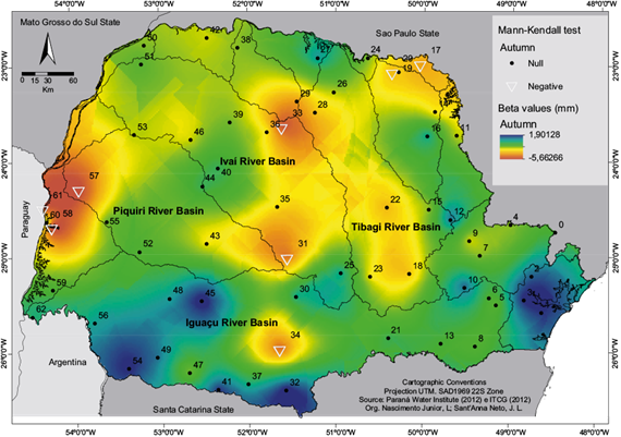
The spatial distribution of these stations suggests a concentration in the extreme west of the area, and another pattern that occurs in the northeast to central-south sectors. The values of β follow this pattern, indicating an increase in precipitation in the eastern sector and part of the southern sector of Paraná State, while negative trends occur below the Tibagi and Ivaí basins.
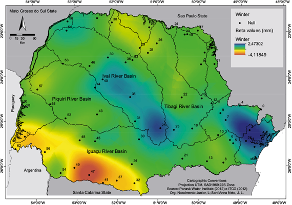
In winter, negative values occur in the extreme southwest of the state, importantly in the west of the Iguaçu River basin and moderately in the north of Paraná State; conversely, they are strongest in the coastal sector and below the Ivaí river basin. According to the Mann-Kendall test, significant trends were not present during the winter (Fig. 5).
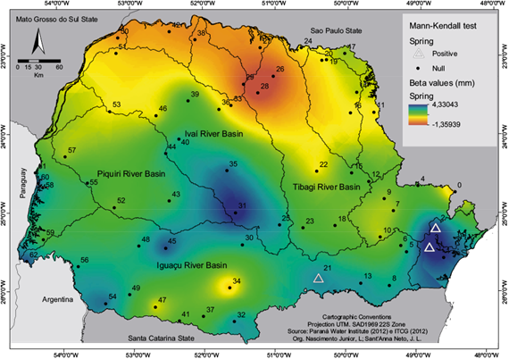
The spring (the quarter that essentially starts the rainy season) presented three series with statistical significance: Antonina, Morretes, and São Mateus do Sul, located in the coastal and southern sectors. The angular coefficients also demonstrated an increase in precipitation in these areas, and a decrease in the north, predominantly in the lower course of the Tibagi River (Fig. 6)
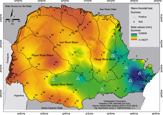
With a more complex pattern, associated with the genesis of rainfall production systems and the high nugget effect (128.733 m), the summer quarter presented eight positive trends in the historical series: Antonina, Adrianópolis, São José dos Pinhais, Rio Branco do Sul, Piraí do South, São Matheus do Sul, Arapongas, Guarapuava, and Rio Bonito do Iguaçu. These localities also coincide with angular coefficient spatialization that occurs in the west sector below the Iguaçu river basin. There was no negative trend in the summer, thus, positive trends are observed throughout the area, and the predominance of the highest positive values is observed in the eastern sector of the state (Fig. 7).
Rainfall trends in the dry season synthesize the sign of gradual decrease in precipitation in the north and west of Paraná State, with two historical series demonstrating a significant negative trend: Cambará and Arapongas. Positive β values occur slightly in the central-south of the state and in the coastal sector (Fig. 8).

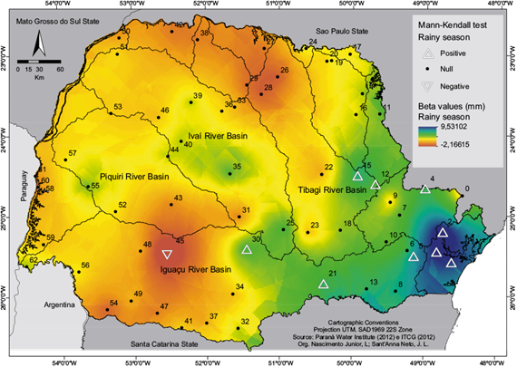
On the other hand, for precipitation detected in the rainy season, a significant negative trend in the western (Rio Bonito do Iguaçu) and eastern sectors (Paranaguá, Antonina, Morretes and Adrianópolis, São José dos Pinhais, Castro, Piraí do Sul, São Mateus do Sul, and Guarapuava, in the continental interior) was observed. It should be noted that there are also positive β values in the majority of this sector of the Paraná State (Fig. 9).
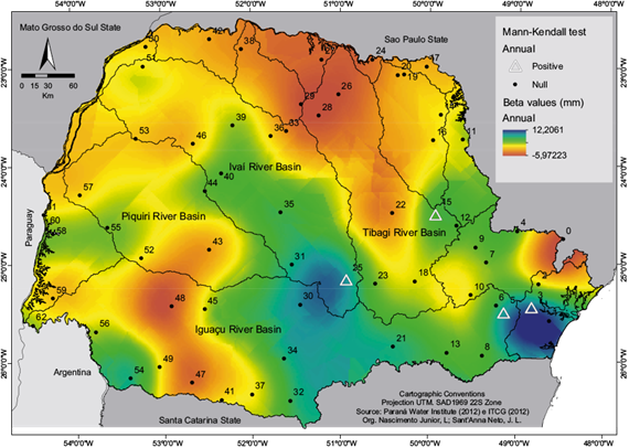
On the other hand, in the annual period, which covers and generalizes all other precipitation results in Paraná State, significant trends were detected in Morretes, São José dos Pinhais, Piraí do Sul, and Prudentópolis (Fig. 10). In this period, the values presented important positive trends in the coastal, central-south, and northwest sectors, while negative trends occurred in the north and west, below the Tibagi and Piquiri basins, and in the low-lying areas of the Ivaí and Iguaçu rivers.
In general, spatial analysis suggests that rainfall variability in Paraná State shows decreases from an important latitudinal-longitudinal gradient, which could be visualized from the variation in values on all the observed scales. A significant contribution arises from the orographic effect, which results in higher rainfall values due to sea breezes from the South Atlantic Ocean. The usual direction of these winds is perpendicular to the coastal sector, forced to ascend the Serra do Mar mountain range very close to the littoral area.
It was also possible to observe spatial connections associated with climate factors. In this case, attention is drawn to the precipitation stations in the coastal areas as well as those located in the watersheds, in the valleys of the large hydrographic basins, and at higher altitudes. This finding can be explained by the topographic relief, which is the main factor for the distribution of rainfall in Paraná, since it drives and impedes air masses and rainfall systems. The joint action of rainfall systems determines both the quantity and intensity of rainfall precipitated on the slopes by means of the orographic factor (Maack, 1981; Monteiro, 1968; Nimer, 1979; Grimm, 2009a, b). In this case, the orographic factor works together with dynamic factors (air masses and other regional atmospheric systems) to show areas with the most important rainfall trends.
7. Discussion
Forty eight statistically significant change points were identified in the time series of precipitation, concentrated in the period from 1991 to 1999, with a maximum of occurrence in 1993 adding up to 27 observations, which corresponds to 56.3% of the total change points detected with statistical significance. The ruptures occurred mainly in the rainy season (33.3%), followed by annual (18.8%), and summer (16.7%) observations.
The periodicity and distribution of the change points could also be related to global- scale factors, specifically to the effect of volcanism on the climate. It can be inferred that the detection of a rainfall change point in these years is also the result of regional and local effects of the eruption of Mount Pinatubo in the Philippines in 1991 and 1992.
Similar results were found in the global precipitation by Iles et al. (2013). These authors verified that volcanism promotes a significant reduction in global mean precipitation, lasting two to three years after the eruption. In general, volcanic activity can release pyroclastic material into the atmosphere, modifying the microphysical properties of clouds. It also reflects incoming solar radiation, causing cooling of the atmosphere, which influences the global climate for months and, in some cases, years (Robock, 2000; Christy and Spencer, 2003; Gu and Adler, 2011).
It was observed that the variability in precipitation is higher during the winter and lower in the annual scale, considering the value of the coefficient of variation. The winter quarter is also the driest in the state, while summer is the rainiest. This relationship also occurs in the comparison between the dry and rainy seasons, which usually characterizes the tropical typology of the most extensive climate in the State of Paraná, that is, the presentation of at least two very distinct precipitation periods (Maack 1981; Monteiro, 1968; Nimer, 1989; Grimm, 2009a, b).
The angular coefficient value provides some initial conclusions for the study of alterations in rainfall variability over the period of analysis. The first conclusion indicates a decrease in rainfall in the less rainy periods (dry season, autumn, and winter), and a rainfall increase in the rainier periods (rainy season, spring, and summer). The signs of the angular coefficient (β) were a parameter for the identification of this process.
Assuming the interpolation of β values and the significance of the trends through the Mann-Kendall test, this analysis contributes to infer the process and tropicalization of rainfall patterns in the state of Paraná, mainly during the rainy season. The results suggest a higher concentration of rain during the wetter period of the year, similar to the results observed by Haylock et al. (2006), Debortoli et al. (2015), Basistha et al. (2007), Shahid (2011), Hasan et al. (2014), and Addisu et al. (2015) in South America, India, Bangladesh, and Ethiopia, respectively.
We suggest that the spatial distribution of trends is more important in regions and areas located in the coastal and southern sectors, since in these areas rains are basically distributed throughout the year, and they present climatic aspects very similar to subtropical climate patterns. In this sense, they differ from the northern sector, which is typically tropical and has two well-defined rainfall seasons (which is a well observed characteristic of climatic transition in the state). Based on this, it is inferred that Paraná (specifically the coastal and southern sectors) has experienced a gradual increase in total precipitation during the recent years, favoring an interpretation of the concentration of rainfall during the rainy season (October to March). This highlights a slow and moderate process of rainfall tropicalization patterns, with a higher rainfall concentration mainly during the rainy (4.03 mm) and summer (2.17 mm) seasons.
Negative precipitation trends were observed in the basins of the Ivaí and Iguaçu, and the coastal sector. A moderate increase was detected in the east and south. There was also a gradual decrease in rainfall in the west and north of the state, as well as specific localities such as Antonina and Morretes on the coast, and Piraí do Sul and Rio Bonito do Sul in the southern sector. These locations showed significant trends in at least three of the observed scales.
It was noted that spring and the rainy season are the most difficult periods to model considering the range, sill and nugget values. This occurs precisely because the rains in both periods can be local (convective) and regional (frontal systems). This impacts directly the spatial dependence of rainfall values at the humid period in tropical areas.
However, the mechanisms of rainfall increase during the positive phase changes of ENSO should be noted. Haylock et al. (2006) suggested a general weakening of the continental gutter in higher latitudes, causing a southward shift in the storm bands during the period.
It should also be noted that, regionally, in the context of the southern region of Brazil, these patterns might also be associated with the causes described by Haylock et al. (2006), who state that trends have two large-scale coupled patterns. In this case, the authors argue that rainfall trends corresponding to canonical coefficients of SSTs influence, show a strong increase of humidity in southern Brazil. In this work, we used more stations and greater details of these trends, showing that the most important signal is observed in the section of Paraná State that exhibits predominately subtropical climates. In the northern sectors, where tropical climates dominate, there are no significant trends. Therefore, we affirm that they are a signal of rainfall tropicalization in the Paraná State, mainly observed in the southern sector.
8. Conclusion
The rainfall data of Paraná State were subjected to the Mann-Kendall test and linear regression and were associated to trends and alterations, mainly observed during the rainy season. The results obtained through geostatistical processing (interpolation of the β values of the linear regression) and mapping of the significant results of the Pettitt and Mann-Kendall tests, corroborate this assertion.
The spatial distribution trends were shown to present good continuity and a markedly defined regionalization. The analysis demonstrates regional decreases in rainfall patterns configured in the northern sector and increases in the southern sector. In addition to the gradual effect of east-to-west orientation, this regional characteristic is associated with important factors of the climate, such as orography, sea winds, and synoptic system directions.
It should be noted that the observations show a gradual and low process of rainfall increase with a slight concentration in the rainy season, mainly in the coastal and southern sector. This enables us to infer a moderate rainfall tropicalization process that is not exclusive of the State of Paraná, but is also observed in research in the context of South America, India, Bangladesh, and Ethiopia. In the context of South America, part of the rainfall trends are also explained by large-scale mechanisms such as ENSO.
The results provide a better explanation of rainfall patterns and variability in the Paraná State and the dynamics of the tropical world and Southern Hemisphere, as well as the impact of trends and climate change on a regional scale.

