


 nova página do texto(beta)
 Inglês (pdf)
 Artigo em XML
 Referências do artigo
 Enviar este artigo por email
 Citado por SciELO
  Similares em
SciELO
Similares em
SciELO 
 Permalink
1. Introduction
The correlation between the total amount of ozone and its meteorological characteristics has been appreciated since the beginning of research on atmospheric ozone. The earlier works of Dobson (Dobson and Harrison, 1926; Dobson et al., 1929, 1946; Dobson, 1931) deal with the connection between synoptic-scale circulation phenomena and total ozone. They show that maximum positive deviations of daily values from the monthly means are generally found to the rear of surface low-pressure areas, while maximum negative deviations are found to the rear of surface highs; also, they found that for many occlusions the maximum positive deviations occur directly over the surface low rather than to the rear. Reed (1950) pointed out that ozone variations are not only caused by chemical processes but also have dynamical origins, expressed by sudden increases in a total amount of ozone accompanying marked increases in tropopause pressure, such as found during the passage of a cold front or depression. Other studies by Reiter and Gao (1982), Uccellini et al. (1985), Shapiro et al. (1982) should also be mentioned. A close relation between potential vorticity (PV) and total ozone is pointed out by Vaughan and Price (1989). Abdel-Basset and Gahein (2003) found that a strong correlation between total column ozone (TCO) and PV remains stable on all levels and the maximum transport of ozone from the stratosphere to troposphere coincides with the maximum developing system, and also with maximum values of PV. The vertical structure of ozone distribution from ozone sounding was studied by Dobson (1973). Dütch (1978) collected ozone soundings data worldwide and presented a climatic analysis of the vertical ozone distribution on a global scale. The direct connection between stratosphere-to-troposphere transport (STT) and peaks in ground-level ozone observations are generally infrequent, with only a small fraction of STT trajectories descending below the mid-troposphere (Viezee et al., 1983; Derwent et al., 1998; Eisele et al., 1999; Stohl et al., 2001; Škerlak et al., 2014). Air from the free troposphere is largely limited to daytime entrainment into the lowest layer of the atmosphere as the planetary boundary layer (PBL) height increases (e.g., Itoh and Narazaki, 2016; Ott et al., 2016); however, the ability for ozone rich air to reach the surface depends on a complex array of factors including the diurnal cycle (Langford et al., 2009, 2012; Itoh and Narazaki, 2016; Ott et al., 2016) and the seasonal cycle of the PBL height (Langford et al., 2015, 2017). Kuang et al. (2017) revealed that the upper air ozone generally increases with increasing temperature or decreasing relative humidity (RH), similarly to the surface. The presence of convective mixing (Thompson et al., 1994; Eisele et al., 1999; Langford et al., 2017), and the elevation of the monitoring station, which is located within the free troposphere, especially with the nighttime collapse of the PBL, can experience direct STT (Langford et al., 2015, 2017). A number of studies has been reported regarding the close link between jet streams and gradients in the total amount of ozone (Reiter and Gao 1982; Shapiro et al., 1982) and the marked signatures on total amount of ozone maps of features such as tropopause folds and cut-off-lows (Uccellini et al., 1985; WMO 1986, Vaughan and Price 1989). However, comparatively little has been understood about the extent to which horizontal variability in the total amount of ozone simply reflects variability in the pressure or structure of the tropopause and the extent to which it reflects variability near the ozone maximum.
The purpose of the present work is to study the relationship between TCO and the development of a cyclonic system that occurred over the Mediterranean area during the period January 18-25, 1981. The study continues with a description of the data used, including TCO and the meteorological reanalysis variables, in section 2, where methodology is also explained. The synoptic situation and the role of polar and subtropical jets are discussed in section 3. The horizontal distribution of TCO and tropopause pressure is presented in section 4. The relationship between TCO and cyclogenesis is quantified in section 5. Discussion of how cyclones may influence the vertical variability of TCO is given in section 6, with final conclusions in section 7.
2. Data and methodology
2.1 Data
ERA-Interim reanalysis data (Dee et al., 2011) is the latest global atmospheric reanalysis data set of the European Centre for Medium-Range Weather Forecasts (ECMWF) with a period from 1979 to 2018 with a 1º × 1º resolution is used for obtaining the TCO and meteorological parameters (http://apps.ecmwf.int/datasets/data/interim-full-moda). It consists of the horizontal wind components (u- eastward, v-northward), temperature (T), geopotential height (z) and ozone mass mixing ratio (OMR) for 37 isobaric levels from 1000 to 1 hPa on regular latitude-longitude grid points with 1º × 1º resolution. Data is available at 0000, 0600, 1200 and 1800 UTC. The extracted domain of study extended from 10.0 to 70.0º N and from 10.0 W to 70.0º E for the period January 18 to 25, 1981. TCO data were directly downloaded due to its units (DU) while OMR data were downloaded for 37 isobaric levels taken as meteorological parameters (the OMR unit is ppm). The inner domain used in our calculations for the present study changes with time to enclose the cyclone during its life cycle (Fig. 2). For each day, the average total amount of ozone was estimated by calculating the average gridded ozone values inside the domain (Fig. 2), which encloses the cyclone cell over the period of study (January 18 to 25, 1981). Therefore, calculations of the total amount of ozone average and meteorological parameters were made only over this domain, to have a better view of the total amount of ozone variations with meteorological parameters.
2.2 Vertical tilt of the wave and northward transport of heat
In this section, we derive the conditions for the westward tilt of a wave with height using the two-level quasi-geostrophic model discussed by Holton (1972). Our problem depends on the correlation between the perturbation thickness (ψ 1 ′ - ψ 3 ′) and meridional velocity ∂(ψ 1 ′ - ψ 3 ′)/ ∂x at 500 hPa. In order to understand this, it is helpful to consider a particular sinusoidal wave disturbance. Suppose that the barotropic and baroclinic parts of the disturbance can be written respectively as
where ψ 1 ′ and ψ 3 ′ represent the perturbations of the stream functions ψ 1 ′ and ψ 3 ′ at 250 and 750 hPa, respectively; x 0 designates the phase difference; ψ 1 ′ + ψ 3 ′ is proportional to the 500 hPa geopotential, and ψ 1 ′ - ψ 3 ′ is proportional to the 500 hPa temperature. The phase angle k x 0 gives the phase difference between the geopotential and temperature fields at 500 hPa. Furthermore, A M and A T are the measures of the amplitudes of the 500 hPa disturbance geopotential and temperature fields, respectively. Using the expressions in Eq. (1) we obtain
From Eq. (2) we can see that for the usual mid-latitude case the relationship between geopotential and temperature fields must be positive if x 0 satisfies 0 < k x 0 < π. Furthermore, the correlation will be a positive maximum for k x 0 = π/2 when the temperature wave lags the geopotential wave by 90º at 500 hPa. It should also be noted here that if the temperature wave lags the geopotential wave, the trough and ridge areas will tilt westward with height, which is observed to be the case for amplifying mid-latitude synoptic systems.
3. Synoptic discussion
Based on the 1000 and 500 hPa charts the life cycle of our cyclone can be divided as following: the first two days (January 18-19) immediately precede the onset of cyclogenesis and can be termed as pre-cyclogenetic period. The third, fourth and five days (January 20-22) are the growth period, and finally, the last three days (January 23-25) are the decay period. This is a typical case of mid-latitude and Mediterranean cyclogenesis (Karacostas and Flocas, 1983; Lionello et al., 2006; Homar et al., 2007; Kouroutzoglou et al., 2011, 2013z). It has long been recognized that cyclogenesis to the lee of the Alps occurs typically with cold air outbreaks crossing the massif from north or northwest and that the primary influence upon cyclogenesis is orographic (Buzzi and Tibaldi 1978; Gomis et al. 1990). This cyclone evolved between 1200 UTC on January 18-25, 1981, while strong cyclogenesis occurred during 1200 UTC on January 20-22, 1981 over the Mediterranean Sea. Figures 1 and 2 show the 1000 and 500 hPa geopotential analysis for the period from January 18-12 to 25-12, respectively.
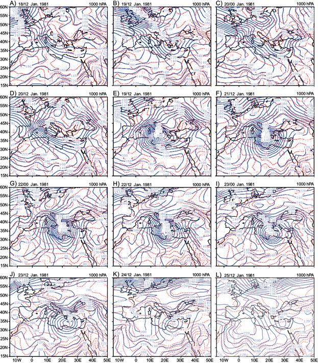
Fig. 1 1000 hPa height contours in 40 gpm intervals (solid) and temperature (dotted) in 5 ºC increments for 1200 UTC on January 18-25, 1981.
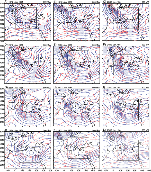
Fig. 2 500 hPa height contours in 60 gpm intervals (solid) and temperature (dotted) in 5 ºC increments for 0000 UTC on January 18-25, 1981.
At 1200 UTC on January 19, Figures 1b and 2b show that a weak low-pressure system with a surface center of 60 geopotential meters (gpm) is located south of Italy and is associated to a baroclinic upper air trough. During the next 24 h, the center of the surface low propagates slowly to the southeastward and deepens to 40 gpm (Fig. 1c). A corresponding upper air trough formed at 500 hPa on January 20 at 0000 UTC was shifted eastward (Fig. 2c). On January 21 at 1200 UTC, Figure 1d shows that the low pressure was deepened to -120 gpm and moved southeast to a point just north of Italy. The development of the upper air trough was accompanied by lee cyclogenesis that started on January 20 at 1200 UTC associated to a cut-off low formed at 500 hPa over the middle of Europe with a center of 5160 gpm. Meanwhile, the Siberian high extended to include most of the northeast of Europe, and a new high-pressure developed over western Europe. On January 21 at 0000 UTC (Fig. 1e), the center of the surface pressure is located over south Italy and the north of Libya with more deepening, where the geopotential height at 1000 hPa reaches -100 gpm. The associated upper air trough at 500 hPa (Fig. 2e) moved southeastward where the geopotential height at its cutoff low was 5200 gpm. Figure 2f (January 21, 1200 UTC) illustrates that the center of the cyclone moved about 15 latitudes southward during 24 h, from 50º N, 15º E on January 20 at 1200 UTC to 35º N, 15º E on January 21 at 1200 UTC. From January 22 at 0000 UTC to January 23 at 000 UTC, the center of the cyclone moved slowly eastward with slight filling and reached 5200 gpm at 500 hPa on on January 23 at 0000 UTC (Fig. 1i). Also, at 1000 hPa the geopotential height at the center of the cyclone increased gradually to reach -40 hPa on January 23 at 0000 UTC (Fig. 1i). During the next two days (January 23-24) the depression started filling and its central pressure increased gradually. On the other hand, the high pressure over the Atlantic extended eastward with a major ridge that joined with the Siberian high on January 22 (Fig. 1h). This means that the subtropical high pressure prevented the northwest cold air (cold advection) from the south and middle of Europe from reaching the cyclone. While the Siberian high extended westward the horizontal extension of the cyclone decreased and moved slowly eastward, becoming a stationary vortex rotating above the northeastern Mediterranean. Finally, the cyclone drifted slowly northeastward and was out of the computational domain after January 25.
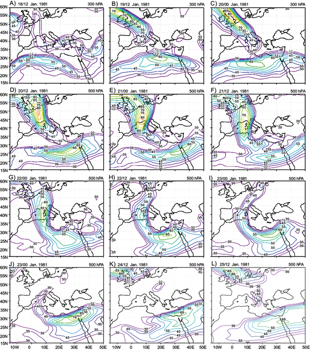
3.1 Behavior of the polar and subtropical jets
It is known that the subtropical (polar) jet has its maximum speed around 200 hPa (300 hPa) (Namias and Clapp 1949; Loewe and Radok 1950; Mohri 1953; Newton 1954; Sutcliffe and Bannon 1954; Defant and Taba 1957; Krishnamurti 1961; Riehl 1962; Palmén and Newton 1969; Keyser and Shapiro 1986; Shapiro and Keyser 1990). Figure 3 displays the horizontal distribution of wind speed (in isotachs) at the 300 hPa level to show the behavior of the polar and subtropical jets during the life cycle of the cyclone. On January 19, 1981 at 1200 UTC (Fig. 3b), the maximum speed of the subtropical jet core was 60 m s-1 and was located over North Africa (northern Libya, Egypt and the northern Red Sea). Its speed at 200 hPa is greater than 60 m s-1 (not shown). The polar jet extended from northwest England to southeast Spain and the north of Italy with a maximum wind speed greater than 70 m s-1 at 300 hPa. Its extension at 200 hPa has a maximum wind speed greater than 65 m s-1 (not shown). On January 20 at 0000 UTC, the subtropical jet moved slightly northeastward and its maximum center, located over Egypt, became greater than 60 m s-1 at 200 hPa. On January 20 at 1200 UTC, the polar jet moved southeastward to amalgamate with the subtropical jet and its maximum value became greater than 70 m s-1 at 300 hPa. On January 21, 1981 at 1200 UTC, the subtropical jet shifted to the southeast while the front of the polar jet reached northern Algeria and the value of its maximum jet was greater than 80 m s-1 at 300 hPa. The subtropical jet weakened at 300 hPa and became stronger at 200 hPa (>70 m s-1), moving eatsward. Beginning on January 22 at 1200 UTC up to January 24 at 1200 UTC the polar jet became weak at 300 hPa and its extension on 200 hPa disappeared. Also, it is noticed that the subtropical jet moved eastward and almost returned to its normal distribution both in speed and direction.
3.2 Tilting behavior
To illustrate the behavior of the vertical axis tilt with the development of our case study (according to the theoretical analysis in subsection 2.2) we computed the perturbation temperature T’ (thickness) and meridional velocity V’, and then calculated the product of these two variables over the computational domain. Fig. 4a shows the time height variation of T’V’ throughout the life cycle of the cyclone, while Fig. 4b illustrates the area average integrated values of T’V’ for the period of interest. It is clear that T’V’ < 0 below 800 hPa from January 18 at 1800 UTC to January 20 at 1200 UTC and above 300 hPa from January 18 at 0000 UTC to January 20 at 0600 UTC. During the growth period (January 20-22) and between the 700-250 hPa layer, the positive values of T’V’ increase up to the maximum from January 20 at 1200 UTC to January 22 at 0600 UTC between 600-250 hPa. During the decay period (January 23-25) the values of T’V’ become negative at most levels. Figure 4b shows that vertically integrated values of T’V’ are positive only during the growth period of the cyclone.
4. Horizontal distribution of TCO and tropopause pressure
In order to highlight the relation between TCO and tropopause pressure (TP), we present here the horizontal distribution of TCO and TP during the period of study. Figure 5 illustrates the horizontal distribution of the TCO evolution during the period from January 18 to 25. Figure 5a displays the values of TCO on January 18 at 1200 UTC. It is clear that the higher values of TCO are located over Eastern Europe (45-55º N, 10-30º E), over the area of the cyclone of interest. According to Figure 5b, within 24 h (January 19 at 1200 UTC) the high values of TCO propagated slightly southeastward associated with the movement of an upper air trough at 500 hPa (Fig. 2b) and its magnitude increased to 450 DU. After 24 h (Fig. 5d) the values of TCO increased (> 450 DU) and the area of higher values of TCO extended to cover northern Italy and mid-Europe, associated with the formation of a cut-off low at 500 hPa (Fig. 2d). On January 21 at 1200 UTC, the polar jet associated to the western flank of the upper air trough moved southeastward, where its front reached Algeria, and advected the cut-off low southeastward to reach southern Italy on January 21 at 0000 UTC and northern Libya on January 21 at 1200 UTC. The horizontal distribution of TCO in Figure 5d-g illustrates that the period of maximum development and deepening of the cyclone (T’V’ > 0) is associated with higher values of TCO (> 450 DU). This situation continued until January 23 at 0000 UTC, when the main core of higher values of TCO coincided with and associated to the 500 hPa low-pressure center. On January 23 at 1200 UTC (Fig. 5i) the trough had extended horizontally and moved slowly eastward. It is interesting to note that the area of maximum values of TCO decreased in association with the area of low values of geopotential height (center of low at 500 hPa). On January 24-25, the upper air trough continued eastward latitudinally and its center moved northward (Fig. 5k, l). It should be noted that the values of TCO decreased. Finally, it can be concluded that there is a strong negative relationship between the geopotential height (thickness of the atmosphere), the TCO, and the higher values of TCO that occur during the growth period of the cyclone.
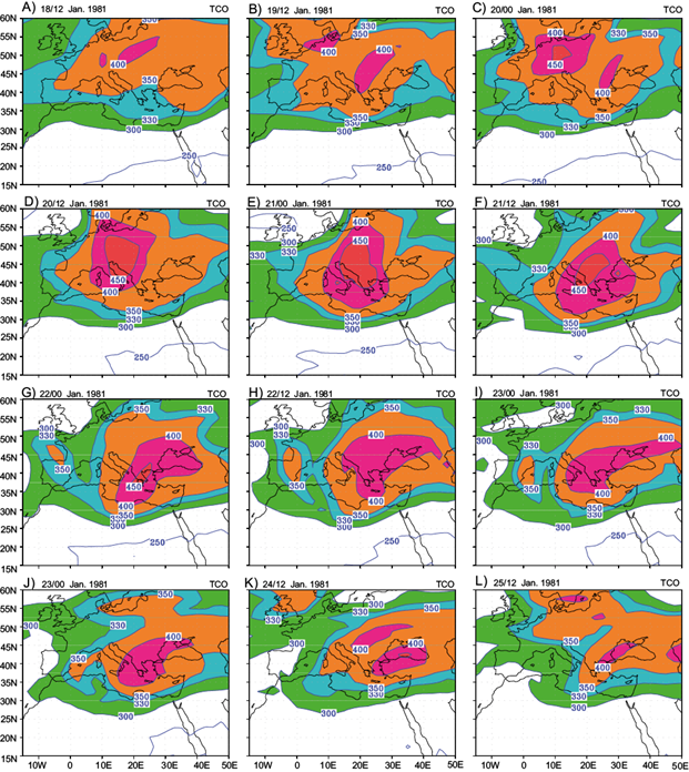
Fig. 5 Horizontal distribution of the vertically integrated values of TCO during the period January 18-25, 1981 (TCO units: DU).
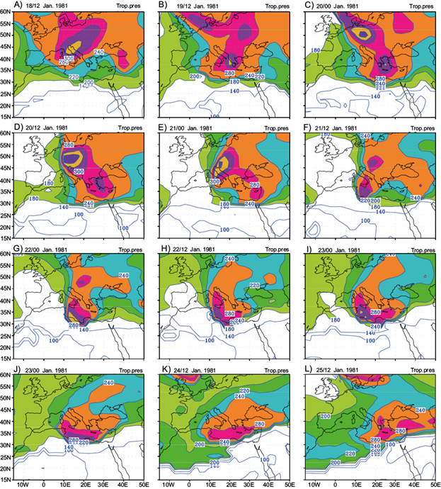
The tropopause is the boundary between the troposphere (a layer of weak stratification) and the stratosphere (a layer of strong stratification) (Holton et al., 1995; Hoinka, 1997, 1998; Highwood and Hoskins, 1998). The global mean height of the tropopause is determined by a balance between the total amount of stratospheric ozone, the surface temperature, and the vertical temperature structure of the troposphere; therefore, changes in any of these values can be expected to lead to changes in the height of the tropopause. The reason for studying the influence of the tropopause pressure on the daily average TCO is that the tropopause forms a boundary surface between comparatively high values of ozone found in the stratosphere and comparatively low values in the troposphere. Figure 6 illustrates the horizontal distribution of the evolution of TP during the period from January 18 to 25. The comparison between Figures 5 and 6 illustrate that there is a very direct connection between the spatial distribution of ozone and the spatial structure of the tropopause pressure. Two important features from Figure 6c are that TCO at northern mid-latitudes (during the life cycle of the study cyclone) is highly variable, and that high TCO is strongly related to high tropopause pressure in the previous day and vice versa.
5. Relationship between ozone and cyclogenesis
It is known that TCO is linked to synoptic-scale meteorological phenomena. In this section we investigate the relation between total amount of ozone, atmospheric thickness, and tropopause pressure throughout the development of our study case.
5.1 TCO and thickness correlation
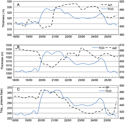
To investigate the relation between TCO and thickness (ΔZ), where ΔZ is the difference between two levels of geopotential height, we divided the troposphere into two layers, the first one between 500 and 1000 hPa, and the second one between 100 and 500 hPa. The TCO and the thickness of the two layers (ΔZ 1 ~ 500-1000 hPa, ΔZ 2 ~ 100-500 hPa) are calculated by averaging all the gridded point values inside the domain that included the cyclone cell throughout the period of study. Figure 7a, b illustrates the daily variation in TCO and the values of TCO, ΔZ 1 and ΔZ 2 , where the maximum values of the total amount of ozone and the corresponding minimum values of ΔZ 1 and ΔZ 2 occurred during the growth period, while the inverse is true during the pre-storm and decay periods. The highest value of TCO during the growth period is about 480 DU on January 21 at 1200 UTC. Finally, it is clear that the relation between the daily values of TCO and the corresponding values of ΔZ 2 is robust, while the relation with ΔZ 1 is weak. The correlation coefficient (r) between the time series of TCO and the corresponding of ΔZ 1 and ΔZ 2 during the period of study is 0.292 and -0.748, respectively. This relationship was used to deduce a linear regression equation relating these parameters.
5.2 Correlation of TCO and tropopause pressure
Figure 7c shows day-to-day variations in the values of TCO and their corresponding tropopause pressure during the period of study. It illustrates a very good correlation between both variables. It is clear that maximum values of the total amount of ozone are associated to maximum values of tropopause pressure and vice versa. It is interesting to note that the maximum values of TCO and maximum values of tropopause pressure occurred during the growth period of the cyclone, from which it can be concluded that when the tropopause descends (i.e., its pressure increases) the fraction of stratospheric air above the location increases, thereby increasing TCO; on the other hand, when the tropopause ascends (i.e., its pressure decreases) there is a corresponding decrease in TCO. The correlation coefficient between TCO and tropopause pressure is 0.289, which indicates that both values are connected.
5.3 Semi-empirical formula for estimating ozone from the thickness
The good correlation coefficients between TCO, thickness (ΔZ 1 and ΔZ 2 ) and tropopause pressure enables us to establish a linear regression equation relating these parameters, which was made by using the time series (32 values) of TCO, ΔZ 1 , ΔZ 2 and tropopause pressure represented in Figure 7. The residual method (Eriksson, 1962) was applied to explore the possibility of forecasting TCO by means of the values of ΔZ 1 and ΔZ 2 and tropopause pressure. The values of TCO during the period of study (January 18-25, 1981) were taken as the dependent variable (predictand) and the corresponding values of ΔZ 1 , ΔZ 2 and tropopause pressure were the independent variables (predictors). In the first step, the correlation coefficient (r) between the values of TCO and ΔZ 1 , ΔZ 2 and tropopause pressure (predictors) is determined. The predictor that has the strongest r with the predictand is used as first predictor, then the regression line and the regression coefficients are determined. The error between the actual and estimated values of TCO are taken as a predictand. In the second step, the above-mentioned error is subjected to the process performed in the first step. The third step is repeated with new predictors (if there are many predictors) until the additional predictor has no significant effect on the predictand and there is no need for any further steps (i.e., the improvement cannot be expected to be very great with adding new predictors). Table I shows the number of steps, the predictor used in each step, the regression coefficients arising from each step (Ai, Bi), the root mean square error (RMSE) and mean absolute error (MAE) arising from the error between the actual and estimated data after each step, and multiple correlation coefficient (r) from a stepwise regression analysis. Table I shows that the total multiple correlations reached 0.94 after using three predictors. This increase in r is associated to a high decrease in RMSE and MAE. The multiple regression equation for predicting values of TCO from the known preceding values of ΔZ 1 , ΔZ 2 and tropopause pressure (TP) can be written as follows:
Table I Regression coefficient (A i , B i ), root mean square error, mean absolute error, and multiple correlations (r) from a stepwise regression analysis.
| Step number | Predictors | Regression coefficients | RMSE | MAE | r | |
| A i | B i | |||||
| 1 | DZ 2 | 3465.095 | -2.9581 | 17.193 | 13.914 | 0.75 |
| 2 | DZ 1 | -590.519 | 1.1292 | 15.004 | 11.713 | 0.87 |
| 3 | TP | -34.666 | 0.1167 | 10.036 | 8.109 | 0.94 |
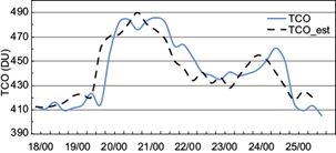
This equation gives valid values of TCO based on the known thickness of ΔZ 1 and ΔZ 2 and tropopause pressure, especially in the cases of deep cyclogenesis. The short data record (32 values) must temper our results. To obtain more statistically reliable results, long data series (large numbers of cases of cyclogenesis) are required. Figure 8 shows day-to-day variations in the values of observed TCO and its corresponding estimated values arising from Eq. (3).
6. Vertical variation of ozone
In this section, the vertical variation of the ozone mixing ratio (OMR) during the study period (January 18-25, 1981) is analyzed. Therefore, average values of OMR at each level over the domain enclosing the center of the cyclone are determined at each time during the period of study (Fig. 9). Generally, it is clear that higher values of OMR occur between 20-5 hPa levels reaching their maxima between January 19-20. OMR values gradually decrease below and above the layer between 5-20 hPa. The semicircle (red color) found in the 250-350 hPa layer represents the height of the tropopause at each time of the period of study (Fig. 9). It is clear that during the pre-storm period the height of the tropopause is steady, and there is no variability of OMR above the tropopause, while below the tropopause there is a significant variability in OMR from the surface up to 450 hPa. With the beginning of the growth period, the height of the tropopause decreased, especially during the period from January 19 at 1800 UTC to January 21 at 1200 UTC with the maximum decrease January 20 at 1200 UTC,, and a sharp change in the vertical gradient of OMR was observed between January 19 at 1800 UTC and January 20 at 0600 UTC in the 100-250 hPa layer. This high decrease of the tropopause height was associated with the high deepening of the cyclone and was accompanied by a significant vertical increase of OMR in the troposphere and stratosphere. The obvious significant increase of OMR started at the stratospheric layer on January 20 at 0000 UTC and then was transported to the tropospheric layer, where a striking change in the OMR was observed between January 20 at 1800 UTC and January 21 at 0600 UTC below 450 hPa. This increase of OMR values below 450 hPa was continuous up to January 23 at 1800 UTC. Figure 9 illustrates also that the height of the tropopause increased and the values of OMR decreased gradually in the troposphere from the beginning of the decay (January 23 at 1900 UTC) to the end of study period. A sharp change in the vertical gradient of OMR between January 23 at 1200 UTC and January 24 at 0600 UTCvbelow 650 hPa was also noticed. After 24/06 and up to the end of the study period January 25 at 1800 UTC an obvious decrease in OMR occured from the surface to 100 hPa, where the greater variability in OMR values obviously occurs, especially in the period of peak cyclonic development.
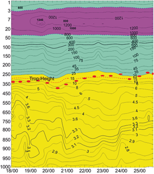
Fig. 9 Vertical profile of OMR (ppm) over the domain containing the center of the cyclone at each level for each time. The semi-circle (red color) in the layer between 400-250 hPa represents the height of the tropopause at each time of the study period.
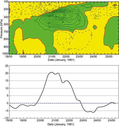
Figure 10a illustrates the time-height variation of the differences of OMR between the average of the domain containing the center of the cyclone at each level and the corresponding monthly average during the period from January 13 to 25. Figure 10a shows that negative values of OMR differences appear above 700 hPa up to the end of the atmosphere during the period from January 13 to 15. The lower level of the negative values raised to 700 hPa on January 18. The higher negative values occurred between the 400 and 10 hPa levels. With the beginning of the cyclone formation and development on January 18, the positive values of the OMR difference appeared above the 400 hPa level on January 19-20. These values increased with height to reach their maxima between 700 and 300 hPa. During the days of maximum deepening and cyclogenesis (January 20-23), the positive values extended downward to reach the 850 hPa level. The increase in positive values continued to be higher in the upper levels to reach maximum values between 300-100 hPa and also between 60-10 hPa. The characteristics of these changes of OMR concentrations from layer to layer are predominantly due to dynamical processes; also, they were attributed to the effect of horizontal advection of ozone from a neighboring region into the column, and by a vertical exchange of air between the high ozone in the stratosphere and the low ozone in trhe troposphere. There is a number of mechanisms to account for the stratosphere-troposphere exchange of ozone, which were discussed by Wei (1986). It is clear that in this case there is a transport of air mass from the lower stratosphere (rich in ozone) to the upper troposphere (stratosphere-troposphere exchange), through which a significant amount of stratospheric ozone penetrates into the troposphere (Levy et al., 1980).
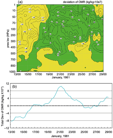
Fig. 10 (a) Time-height variation of the differences of OMR between the average of the domain containing the center of the cyclone at on January 21 at 1200 UTC and the corresponding monthly average. (b) Total vertical average values of OMR differences.
Figure 10b shows the vertical average values of the differences of OMR between the averages of the domain containing the center of the cyclone at each level and the corresponding monthly average for the period from January 13 to 29. The figure illustrates that there is a decrease of OMR from the monthly average during the period from January 13 at 0000 UTC to January 16 at 1200 UTC. With the beginning of the formation of the cyclone the difference between the daily values of OMR from the corresponding monthly average becomes positive and increases gradually to reach its maximum values on January 20-22, associated to the maximum deepening of the cyclone. The comparison between Figures 10b and 4b illustrates that the negative and positive values of the OMR difference are associated with T’V’ < 0 and T’V’ > 0, respectively, which means that the values of ozone increase with the formation and development of the cyclone.
7. Summary and conclusions
The relation between TCO and the development of a cyclonic system that occurred in the period January 18-25, 1981, has been studied. It was found that during the pre-storm period the area average integrated values of T’V’ are negative, associated to lower values of TCO, while with the beginning of the growth period (January 20-22) the area average integrated values of T’V’ are positive, associated to higher values of TCO. During the decay period, the area average integrated values of T’V’ become negative and are associated to lower values of TCO. This illustrates that there is a strong relationship between the cyclogenesis and development of the case study and the values of TCO.
The relation between TCO and the thickness between 1000-500 hPa, 500-100 hPa and the tropopause pressure has been investigated during the period of cyclone development (January 18-25, 1981). A strong correlation was found between TCO and the above-mentioned parameters, especially during the periods of maximum development of a cyclonic system. The residual method has been used to derive a linear regression equation that relates TCO with the thickness and tropopause pressure. This equation was deduced from the short data record of 32 values representing the period of study and must be taken as preliminary, subject to further detailed examination. To obtain more statistically reliable results, long data series (large numbers of cases of cyclogenesis) are required.
The daily variations of TCO based on the vertical distribution of OMR (37 levels) have been studied throughout the period of interest. It was noted that during the pre-storm period there were no vertical changes in OMR values above the tropopause, while below the tropopause a small vertical changes in OMR values occurs from the surface up to 350 hPa. With the beginning of the growth period, the height of the tropopause decreased, especially during the period from January 19 at 1800 UTC to January 21 at 1200 UTC, with a maximum decrease on January 20 at 1200 UTC. This high decrease of the tropopause height, which was associated to high deepening of the cyclone, was accompanied by a significant vertical increase of OMR in the troposphere and stratosphere. The obvious significant increase of OMR started at the stratospheric layer on January 20 at 0000 UTC and was then transported to the tropospheric layer, persisting throughout the period from January 21 at 0000 UTC to January 23 at 1800 UTC. With the beginning of the decay period (January 23 at 1900 UTC), the height of the tropopause increased and the values of OMR decreased gradually in the troposphere until end of study period. Obviously, the greater variability in OMR values occured in the layer from the surface to 100 hPa, especially during the peak of the cyclone development. The analysis of the time-height variation of the differences of OMR between the average of the domain containing the center of the cyclone at each level and the corresponding monthly average illustrates that during the days of maximum deepening and cyclogenesis the positive values of OMR extended downward to reach the 850 hPa level. This means that there is a transport of air mass from the lower stratosphere (rich in ozone) to the upper troposphere (stratosphere-troposphere exchange), through which a significant amount of stratospheric ozone penetrates into the troposphere.

