


 text new page (beta)
 English (pdf)
 Article in xml format
 Article references
 Send this article by e-mail
 Cited by SciELO
  Similars in
SciELO
Similars in
SciELO 
 Permalink
1. Introduction
Dangers related to floods may be attributed particularly to a factor or a combination of factors. An extreme or abundant rainfall level in a short period of time may lead to sudden floods in an area. In the same way, a prolonged period with heavy rainfalls may trigger flooding. For instance, a 75-mm rainfall that lasts four days may have more significant side-effects if that amount falls within 10 h during three days, rather than more evenly spread over the four days.
The analysis of trends and climate extremes variability has received increasing attention recently. However, the availability of quality data on a daily basis over long periods, as required for the analysis for extremes variations is so far the major hindrance (Easterling et al., 2000). However, avoiding water damage due to paying appropriate attention to extreme rainfalls, namely maximum daily rainfalls, the trends within one hour on monthly or decadal basis. The daily scale is considered in this study in order to meet the requirements of monitoring networks optimization and to increase precision estimates inherent to the design of hydraulic structures.
The behavior of maximum levels may be described through the three distributions of maximum levels, namely Gumbel, Fréchet and the negative distribution of Weibull, as suggested by Fisher and Tippett (1928). The first study regarding the distribution of maximum values was probably performed by Fuller in 1914 (Nadarajah, 2005). Thereafter, many researchers considered the distribution of extreme rainfall values in different regions of the world: Oyebande (1982) in Nigeria; Rakhecha and Soman (1998) in India; Withers and Nadarajah (2000) in New Zealand; Crisci et al. (2002) in Italy; Parida (1999) in Greece; Naghavi and Yu (1993), Segal et al. (2001) and Nadarajah (2005) in the United States; Kieffer and Bois (1997), Neppel et al. (2007) and Mora et al. (2005) in France, and Zolina et al. (2008) in Germany. The daily maximum rainfall distribution for 92 stations in the sate of Louisiana, USA, follows the log-Pearson type 3 distribution (Naghavi and Yu, 1993).
In Algeria, the Gumbel distribution is frequently used to study extreme values of rainfalls and discharges. These studies are used to determine the size of hydraulic structures (dams, dikes, channels) that are used to protect from flooding and at the same time ensure the supply of potable water to the population. Koutsoyiannis (2004) showed that applying the Gumbel distribution may lead to a bad assessment of risk due to an underassessment of the largest extreme values of rainfalls, especially when some decadal series do not have the same distribution than the real one. This suggests wrongfully that the Gumbel distribution is the appropriate model. The statistic prediction approach in hydrology consists in a local frequential analysis based on probabilistic calculations using the history of events to predict the frequencies of future appearances. This analysis allows, for each of the samples studies, the assessment of quantiles that correspond to the return periods generally used in hydrology, namely 10-yr, 100-yr, etc.
The approach based on regional frequency analysis methods used to allow an overall description of the spatial structure of different hydrologic phenomena in a region. Those methods were initially developed for the assessment of flood flows (e.g., Darlymple, 1960; Cunnane, 1987; Gupta and Waymire, 1998; Ouarda et al., 2001). Their application range was extended afterwards to precipitations. Thus, incorporating regional information for rainfall frequency analysis becomes more important.
The main goal of developing a regional frequency analysis method is to search for a regional distribution model of annual maximum daily rainfalls that will allow the assessment of rainfall quantiles in sites that do not have much data or have no data at all. This relies in the definition of homogeneous regions within the study region and the validation of homogeneity for each defined region. A procedure based on L-moment ratios will be used to define homogeneous regions. Inter-site variability will be then assessed using simulations to test the statistic homogeneity. The regional analysis procedure thus consists in identifying the regional distribution and assessing its parameters for each defined region.
The ascending hierarchical classification (AHC) method will be used to determine the homogeneous regions that will be confirmed later by the L-moments method. This regionalization will be used to choose the theoretical model best fitted to maximum daily precipitations series. The same procedure of establishing homogeneous zones and then applying the L-moments method, was used in Turkey by Yurekli (2009).
The local approach (Habibi et al., 2013; Boucefiane et al., 2014) led to the selection of the generalized extreme value (GEV) distribution as the best model to adjust the maximum daily precipitation in the steppe area of northwestern Algeria. The absence of this approach is related to the assessment of frequential values for stations that have short series or many gaps. This inability may be prevented by adopting the regional approach through the development of a regional fitting model with the capacity to calculate the daily rainfalls of these stations. To evaluate the pertinence of the regional approach, quantiles estimated from this approach and those estimated from the local approach for different return periods at certain number of stations are compared.
2. Materials and methods
2.1 Study area
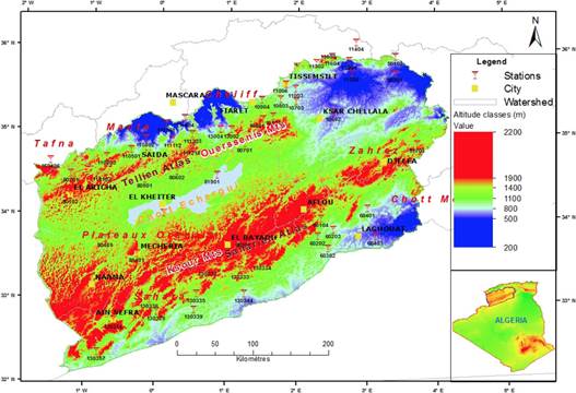
The study region is part of a vast geographic unit, the steppe area, located to the west of the Algerian highlands. It is a semi-arid zone positioned between the edges of the Tell Atlas (Tlemcen and Ouarsenis mountains), to the north, and the Saharan Atlas (Ksours mountains), to the south (Fig. 1). Its coordinates are 1º 30’ E to 4º 0’ W, and 32° 20’ S to 36° 0’ N, covering a surface of 138 500 km2. It is characterized by a wide endoreic expanse where discharges converge on the salt lakes lined in strings and the stream system is not well developed. Most of the wadies originate on the Tell Atlas crests and flow to the south into the Chergui salt lake.
The area fits in the arid and moderate bioclimatic stage with cool winter (Emberger, 1942). It constitutes a buffer zone between western coastal Algeria and Saharan western Algeria. Rainfall is not very abundant, but it often occur as violent storms on a regular basis during nine months of the year. The pluviometric mean is 318 mm spread over 47 days (Benslimane et al., 2015).
Rainfall recorded on all pre-desert subregions of the western steppes is the weakest in the western Algeria region. An isohyets map drawn by the National Water Resources Agency (ANRH) shows that rainfall in this area varies from 100 to more than 300 mm yr-1. The highest precipitation occurs in the mountainous area located to the north aside the Tlemcen and Saida mountains. Annual accumulation ranges from 200 to 300 mm on the high plateaus and the south, and up to more than 400 mm on the reliefs. The areas which received less rainfall (100 to 200 mm) are those ubicated in the salt lakes. Gross time series analysis shows that the driest spells were recorded in 1983 at the Slim station (47.2 mm), to the east; in 1985 at the Ain Skhouna station (77.7 mm), located northeast of the Chergui salt lake, and in 2004 in the north faces of the Saharan Atlas, at the Mecheria station (116 mm). The most humid years were 1971 and 1972 with about 312 mm of precipitation at the Slim station and 292 mm at the Ain Mehdi station. The most humid year recorded at the Mecheria station was 2008 (430 mm).
2.2 Data
The selection of stations was conducted based on the need of necessary information for the study regarding the length and spatial distribution of observational series of these stations within the study region. Concerning the altitude, the highest stations are those of Ain El Orak and Kherba Ouled Hellal, located at 630 masl. The rainfall gauge network of the steppe region of western Algeria includes more than 150 stations managed by the ANRH. These stations are very unequally spread from north to south and west to east on the region. The highest density of the network is found in the north; the density in the south is lower, and the salt lakes region is practically devoid of stations. For the study, 65 rainfall gauge stations that have more than 20 yrs. of observations and short gaps were selected (Fig.1). The basic characteristics of these rainfall gauge stations are presented in Table I.
Table I Gauge stations and their characteristics.
| N° | Code | Station | Coordinates (UTM) | Elevation | Period of data | Record | |
| X (m) | Y (m) | (m) | collection | length (yrs.) | |||
| 1 | 010502 | ZMALET EL AMIR AEK | 437056 | 3861500 | 820 | 1969-2008 | 31 |
| 2 | 010602 | AIN ZERGUINE | 455726 | 3903140 | 786 | 1922-1947 | 22 |
| 3 | 010701 | AIN BAADJ | 376314 | 3898321 | 1025 | 1974-2009 | 28 |
| 4 | 010703 | RECHAIGA | 407273 | 3918283 | 830 | 1931-2010 | 53 |
| 5 | 010706 | SIDI BOUDAOUD | 443357 | 3913226 | 710 | 1974-2011 | 35 |
| 6 | 010803 | MEHDIA | 386680 | 3921193 | 903 | 1967-2010 | 40 |
| 7 | 010901 | SOUGUEUR | 363253 | 3894657 | 1120 | 1914-2009 | 84 |
| 8 | 010904 | DAHMOUNI TRUMULET | 361573 | 3919865 | 878 | 1970-2010 | 38 |
| 9 | 011003 | COLONEL BOUGARA | 406122 | 3934937 | 820 | 1968-2010 | 38 |
| 10 | 011004 | KHEMISTI | 407008 | 3947085 | 928 | 1968-2011 | 42 |
| 11 | 011006 | TISSEMSILT | 393238 | 3940825 | 858 | 1976-2009 | 30 |
| 12 | 011104 | AIN BOUCIF | 513681 | 3971260 | 1250 | 1923-2008 | 57 |
| 13 | 011206 | CHAHBOUNIA | 464115 | 3932963 | 665 | 1933-2011 | 32 |
| 14 | 011208 | BOUGHZOUL | 479984 | 3955814 | 643 | 1948-2010 | 60 |
| 15 | 011301 | KSAR EL BOUKHARI | 477483 | 3971671 | 630 | 1970-2011 | 31 |
| 16 | 011302 | DERRAG | 444939 | 3973521 | 1160 | 1914-2011 | 63 |
| 17 | 011404 | ZOUBIRIA MONGORNO | 486509 | 3996343 | 1000 | 1915-2011 | 74 |
| 18 | 011603 | BORDJ EL AMIR AEK | 434025 | 3969004 | 1080 | 1922-2011 | 73 |
| 19 | 011604 | KHERBA OD HELLAL | 454850 | 3976940 | 1290 | 1968-2009 | 41 |
| 20 | 013002 | FRENDA | 321259 | 3881018 | 990 | 1967-2009 | 39 |
| 21 | 013004 | AIN EL HADDID | 307155 | 3881055 | 829 | 1967-2010 | 41 |
| 22 | 050102 | CHELLALAT EL ADAOURA | 537949 | 3977185 | 1004 | 1955-2011 | 40 |
| 23 | 050201 | DRAA EL HADJAR | 538531 | 3955233 | 726 | 1968-2011 | 34 |
| 24 | 051703 | SLIM | 567480 | 3861498 | 1070 | 1967-2008 | 36 |
| 25 | 052002 | AIN RICH | 600594 | 3837441 | 944 | 1953-2007 | 32 |
| 26 | 052102 | BORDJ L’AGHA | 628275 | 3861643 | 795 | 1971-2007 | 29 |
| 27 | 060104 | SEKLEFA | 439810 | 3762787 | 995 | 1972-2007 | 28 |
| 28 | 060202 | AIN MAHDI | 435640 | 3739299 | 985 | 1969-2013 | 32 |
| 29 | 060203 | TADJEMOUT-2 | 456266 | 3748238 | 885 | 1926-1997 | 66 |
| 30 | 060302 | EL HOUITA | 449192 | 3722860 | 900 | 1970-2005 | 25 |
| 31 | 060401 | SIDI MAKHLOUF | 501343 | 3776103 | 900 | 1967-2007 | 32 |
| 32 | 060403 | KSAR EL HIRANE | 512235 | 3739077 | 710 | 1969-2005 | 29 |
| 33 | 080102 | EL ARICHA | 107915 | 3794637 | 1250 | 1901-2010 | 50 |
| 34 | 080201 | EL AOUEDJ (Belhadji B,) | 108284 | 3823484 | 1075 | 1970-2009 | 39 |
| 35 | 080401 | MEKMENE BEN AMAR | 154083 | 3737180 | 1050 | 1970-2005 | 29 |
| 36 | 080501 | MARHOUM | 206461 | 3815250 | 1115 | 1973-1993 | 20 |
| 37 | 080502 | MOULAY LARBI | 226518 | 3837925 | 1155 | 1942-2009 | 43 |
| 38 | 080602 | KHALFALLAH | 248755 | 3826173 | 1100 | 1942-2004 | 42 |
| 39 | 080604 | MOSBAH | 233430 | 3811978 | 1075 | 1943-2010 | 31 |
| 40 | 080606 | MAAMORA | 271195 | 3840179 | 1148 | 1975-2010 | 29 |
| 41 | 080701 | MEDRISSA | 339264 | 3862568 | 1105 | 1932-2010 | 60 |
| 42 | 080902 | STITTEN | 336621 | 3736799 | 1410 | 1973-2010 | 33 |
| 43 | 081401 | MECHERIA | 196070 | 3716871 | 1167 | 1907-2010 | 90 |
| 44 | 081502 | BOUGTOB | 230978 | 3770456 | 1000 | 1943-2009 | 41 |
| 45 | 081901 | AIN SKHOUNA CAMP | 302489 | 3820733 | 1000 | 1947-2004 | 30 |
| 46 | 110102 | RAS ELMA | 149876 | 3823858 | 1094 | 1919-2010 | 66 |
| 47 | 110203 | EL HACAIBA | 155972 | 3846023 | 950 | 1970-2010 | 38 |
| 48 | 110501 | MERINE | 188824 | 3854817 | 951 | 1970-2009 | 35 |
| 49 | 110802 | DAOUD YOUB | 207072 | 3869290 | 657 | 1927-2010 | 68 |
| 50 | 111112 | HAMMAM RABI | 242997 | 3868708 | 695 | 1970-2010 | 30 |
| 51 | 111201 | OUED TARIA | 234990 | 3889090 | 480 | 1908-2010 | 90 |
| 52 | 111203 | AIN BALLOUL | 269475 | 3874698 | 1014 | 1967-2006 | 31 |
| 53 | 111210 | TAMESNA | 268186 | 3858643 | 1005 | 1970-2009 | 33 |
| 54 | 111404 | AOUF M.F. | 259823 | 3895983 | 990 | 1928-2010 | 60 |
| 55 | 130329 | BOU SEMGHOUM | 221378 | 3639873 | 985 | 1969-1995 | 26 |
| 56 | 130332 | AIN EL ORAK | 289588 | 3698626 | 1290 | 1970-1995 | 25 |
| 57 | 130333 | GHASSOUL | 332893 | 3694597 | 1250 | 1970-1996 | 24 |
| 58 | 130334 | SIDI AHMED BELABBES | 361336 | 3706617 | 1210 | 1970-1995 | 23 |
| 59 | 130335 | ARBA TAHTANI | 274279 | 3663350 | 600 | 1950-1995 | 30 |
| 60 | 130336 | ASLA | 212413 | 3656412 | 1170 | 1969-1995 | 26 |
| 61 | 130339 | EL ABIOD SIDI CHEIKH | 270620 | 3642048 | 903 | 1911-1994 | 42 |
| 62 | 130344 | BREZINA | 337906 | 3663276 | 927 | 1971-1994 | 23 |
| 63 | 130356 | AIN SEFRA ANRH | 164789 | 3628600 | 1072 | 1972-1995 | 22 |
| 64 | 130357 | DJENIENE BOU REZG | 141667 | 3586696 | 1019 | 1972-1996 | 20 |
| 65 | 160406 | KHEMIS OULD MOUSSA | 81904 | 3841795 | 1000 | 1924-2010 | 47 |
2.3 L-moments
To validate the homogeneity of a region in terms of L-moments relationships, the discordance test proposed by Hosking and Wallis (1993) will be used:
be u the vector containing the values t, t 3 and t 4 for the site i, where the exponent T refers to a vector or a matrix, and
In the equation below N is the sample size of each group and S -1 the invert of the matrix S.
Hosking and Wallis (1997) proposed the criterion D i ≥ 3 to exclude a station from the homogenous region. Inter-site relationship is used to identify the homogenous sites with a similar frequency distribution. The heterogeneity test H i compares samples of L-moments relationships with the parameters of the Kappa distribution; it measures the heterogeneity between the sites of the same region. Hosking and Wallis (1997) proposed the following statistic:
where μ v etσ v are the mean and the standard deviation of N sim of the simulated values of V 1 .
V 1 is calculated by the following relationship:
Simulations are done by using a flexible distribution with the regional mean of L-moments ratios 1, τ, τ 3 , t and τ 4 . Following Hosking and Wallis (1993), 1997), we used the distribution with four Kappa parameters with the following quantiles function in the simulations (Hosking, 1994):
In order to get reliable values of μ v and σ v , the number of simulations N Sim will be great. The region is considered as acceptably homogenous if H < 1, possibly heterogeneous if 1 ≤ H <2, and certainly heterogeneous if H ≥ 2. H1 is the homogeneity measurement in terms of L-CV; H 2 is the homogeneity measurement in terms of L-CS, and H 3 is the homogeneity measurement in terms of L-CK.
The statistic Z (Hosking and Wallis, 1991) determines to which extent the L-skewness and L-kurtosis simulation of a fitted distribution correspond to the regional mean of L-skewness and L-kurtosis values, obtained from the data observed. In this work, the quality criterion for fitting is defined by the statistic ZDIST depending on the various candidate distributions:
where t 4 R is the mean value of t 4 relating to the data of the relevant region, and B 4 and are the bias and standard deviation of t 4 , respectively, and they are defined as follows:
where N Sim is the number of regional data simulations fixed generated by using a Kappa distribution (Hosking and Wallis 1988), and m is the m th region simulated by obtaining a Kappa distribution.
The fitting is adequate if ZDIST is sufficiently close to zero. |Z DIST | ≤ 1.64 If it can be said that the fitting is reasonable.
If more than a candidate distribution is acceptable, the one with the smallest |ZDIST| is considered as the most appropriate. Furthermore, the L-moments ratio diagram is also used to identify the best distribution by comparing its proximity to the combination of L-skewness and L-kurtosis of the L-moments ratios.
The idea behind the use of the L-moments diagram is based on the operating of unique combinations of skewness and excess coefficients, to graphically identify the function that is closest to the studied sample distribution. To choose the most pertinent probability distribution, the use of existing regional works, or the L-moments diagram, is recommended (Ben-Zvi and Azmon, 1997; Chen et al., 2006). When the scatter of L-moments ratios is close to a large number of probability distributions, the mean of the L-moments ratios of observations series is placed on the L-moments diagram and the closest distribution is chosen as the best distribution (Kumar et al., 2003; Chen et al., 2006).
The candidate distributions which will be used to this effect are:
General logistic (GLO), particularly the case of Kappa distribution with the parameter h = -1.
Generalized extreme value (GEV), particularly the case of Kappa distribution with the parameter h = 0.
Generalized normal (GNO).
Gaucho, particularly the case of Kappa distribution with the parameter h = 0.5.
Generalized pareto (AMP), particularly the case of Kappa distribution with the parameter h = 1.Pearson 3 (P3).
Kappa distribution (KAP).
The condition to have a homogenous region is that all sites may be described by a probability distribution that has common distribution parameters; thus, all sites of a homogenous region have a common regional curve of frequency, which is called regional growth curve (L-RAP, 2011).
After determining the most appropriate frequency distribution model for each of the three homogenous groups, the quantiles for different return periods are estimated by using the rain index method. This procedure supposes that data of maximum daily rainfalls of different sites in a homogeneous group have the same statistic distribution, except for a scale parameter specific to a site or an index factor (Dalrymple, 1960). The scale factor is considered as the rain index. The quantile of a homogenous group is estimated by the following equation:
where P i (F) is the value of the daily maximum rainfalls at station i with a non-exceedance probability F; μ ̂ i is the sample mean to this station, and p(F) is the dimensionless quantile with exeedance probability given by F. The totality (F) values for 0 < F < 1 result from the regional growth curve. This approach was used in many countries following the example of Malekinezhad and Zare-Garizi (2014) in Iran, Yurekli et al. (2009), in Turkey, Ngongondo et al. (2011) in Malawi, and Martin (2015) in Canada. This approach is based upon the flood-index method (Darrlymple, 1960). The priori assumption that data are independent and identically distributed as per the same statistic law should be made (St-Hilaire et al., 2003). The same flood index is commonly used to develop the regional models of frequency for the sites where hydrologic information is not sufficient for reliable information of extreme events (Cunane, 1987; Watt, 1989; Portela and Dias, 2005; Saf 2009; Nyeko-Origami et al., 2012).
Uncertainty is detailed after quantiles estimation for a station in each group through regional analysis (Eq. 4). Uncertainty is evaluated by using the bias (BIAS) and the square root of the root mean square error (RMSE) for each homogenous group:
Pmax i R and Pmax i L represent the quantiles of the return period T estimated for the station i, respectively, for the GEV distribution regional and local parameters. N is the number of stations of each homogenous group.
Both MAE and RMSE express the average model prediction error in units of the variable of interest. Both metrics can range from 0 to ∞ and are indifferent to the direction of errors; they are negatively-oriented scores, which means lower values are better. The more that BIAS and RMSE values come closer to 0, both the precision of the value estimated and the method are better.
L-moments present weaknesses and strengths (El Adlouni et al., 2003):
The robustness of L-moments faced with large values may exclude the information regarding extreme values (Bernier, 1993). According to Klemes (2000), this technique favors the choice for the GEV distribution. Ben-Zvi and Azmon (1997) maintain that the L-moments diagram does not provide the best fitting distribution among the acceptable ones.
On the other hand, sample variability affects L-moments less (Vogel and Fennessey, 1993) and they are more robust in the presence of outsiders (El Adlouni et al., 2003).
2.4. Ascendant hierarchical classification
The ascendant hierarchical classification is a mode of classification that consists in aggregating first the most similar individuals, then slightly less similar observations or groups of observations, and so on until the trivial grouping of the whole of the sample.
Let there be a set of n individuals characterized by p variables X 1 ,X 2 ,X 3 ,……….,X p that we want to group in k classes or subclasses as homogeneous as possible according to defined criteria. To do this, according to each criterion, the closest individuals that are connected to each other must be searched. Gradually, all the individuals following a hierarchical tree or dendrogram are grouped together. This dendrogram presents the composition of the different classes as well as the order in which they are formed.
Individuals in the dendrogram are organized hierarchically according to the distances that separate them. The type of distance between individuals is selected depending on the data studied. Among others, the Euclidean distance, which is the type of distance most commonly used, must be distinguished, since it is simply a geometric distance in a multidimensional space. The Euclidean distance is given by the following equation:
where I i is the individual of day i, I j is the individual of day j, and X ik is the observation of day i at the station k.
Performing an ascending hierarchical classification therefore consists in partitioning all the elements of the population into subsets such that each subset is well differentiated from the others. For this, an index of aggregation (distance between groups or between an individual and a group) is fixed taking into account aggregation criteria such as single linkage (minimum distance), complete linkage (maximum distance), and Ward’s method, to minimize the sum of squares of all the pairs of classes that can be formed at each step.
By cutting the tree (dendrogram) at a significant jump in the aggregation index, a good score can be obtained because the individuals grouped below the cut are close to each other, while those grouped after the cut are far apart.
3. Results and discussion
3.1. Test for stationarity and independence
The software HYFRAN (Bobée et al., 1999) allows to achieve a full frequential analysis for any variable for which one has observations: independent (absence of self-correlation) and identically distributed (homogeneity, stationarity and absence of outsiders). Thus, the study of the series independence and stationarity precedes the series distribution stationarity of the maximum daily rainfalls. Statistic tests of stationarity (Kendall) and independence (Wald-Wolfowitz) are applied to each series. Mann-Kendall is a non-parametric statistic test to detect trends in the time series devoid of seasonality. Both tests used are accepted for all stations at a 5% threshold (Table II). From these results, representativeness of annual maximum daily rainfalls series is accepted.
3.2. Discordancy, homogeneity, and goodness-of-fit tests
Regional estimation of hydrometeorological variables is necessary to specify the asymptotic behavior of the annual maximum daily rainfalls distribution, to reduce the sampling influence on short series, and particularly to remedy the data shortage in sites devoid of measuring stations (Muller, 2006). The first stage for this procedure is the decomposition of the study region into homogeneous groups of stations. The methods commonly used in hydrology to create homogeneous groups of stations are generally based on the determination of regional indices and multivariate analysis (Muller, 2006; Meddi and Toumi, 2015). The variables belonging to a homogeneous region result from the same population; thus, they follow the same probability distribution and share the same parameters. To validate the homogeneity of a region in terms of L-moments, the statistic homogeneity test proposed by Hosking and Wallis (1993) will be used. Once the regions limits are fixed, the homogeneity of the sites within the region can be validated. This step often consists in calculating the coefficients of variations, asymmetry and kurtosis for every site in the region and then comparing their variability with that of the homogeneous regional model (Schaefer, 1990; Cong et al., 1993; Alila, 1999; Sveinsson et al., 2000).
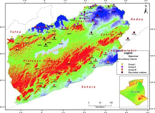
Regional homogeneity was tested first by using discordance (D i ) and heterogeneity (H i ) tests. The results showed heterogeneity on the whole area with regard to L-Cv and L-Cs. If the variable studied (namely annual maximum daily rainfalls) does not follow the same probability distribution with the same parameters, it does not belong to the same population (Table III). Therefore, the assembly of stations in homogenous groups is necessary. To this end, we used ascending hierarchical classification, which highlighted three distinct groups (Fig. 2). Station distributions in homogeneous groups (Fig. 2) are due to the fact that such groups are naturally separated under the effect of their exposure to winds; the stations that coincide with this direction of exposure to winds receive more rainfalls. This is the case of stations in group I. On the other hand, stations in the second group are situated under shelter, which makes them receive less rainfalls despite the fact that they are located to the north, where the mountain barrier hinders the advance of dominating humid air masses, which follow a north-west direction causing abundant rainfalls. Finally, the third group is located at the meeting point of two mountain chains, in a zone characterized by flat topography where rainfall is generally stormy.
Table III Result of the homogeneity test for the different groups.
| Group | Number of stations | Obs Number | Di min - max | H1 | H 2 | H 3 |
| Set | 65 | 2338 | 0.07 - 6.2 | 10.51 | 1.66 | -0.32 |
| Group 1 | 23 | 909 | 0.06 - 2.45 | 0.53 | -0.95 | -1.13 |
| Group 2 | 18 | 717 | 0.01 - 1.88 | 1.31 | -0.72 | -1.13 |
| Group 3 | 14 | 409 | 0.05 - 2.31 | 0.03 | -0.44 | 0.43 |
To evaluate the degree of homogeneity of each group, series of 1000 simulations of maximum daily precipitation as per the GEV distribution were carried out. Results of the homogeneity tests for each group in terms of L-moments ratio are presented in Table III. To validate the homogeneity of the three groups in terms of L-moments, the D i discordance and heterogeneity tests proposed by Hosking and Wallis (1993) were taken into account. The discordance test indicates if rainfall stations in the same group are significantly different from others. This statistic is calculated for the three groups. The results show that this test is concluding in the case of the three groups. The critical value of D i = 3 is not exceeded (Table III).
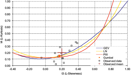
Furthermore, homogeneity tests H 1 , H 2 and H 3 estimate the degree of homogeneity for a given group to determine if a specific group is homogeneous (Table III). These confirmations are necessary to choose the statistic model of regional fitting. The results of homogeneity tests for each group in terms of L-moment ratios are presented in Table III, where it is shown that group I (14 stations) is homogeneous in terms of L-Cv, L-Cs and L-Ck (H < 1) (Fig. 3).
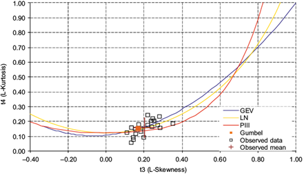
Group II is homogeneous in terms of L-Cv, L-Cs and L-Ck (H < 1). This group consists of 23 stations which are represented in Figure 4.
Group III is homogeneous in terms of L-Cs and of L-Ck (H < 1), but probably heterogeneous in terms of L-Cv. This group consists of 18 stations, as shown in Figure 5.
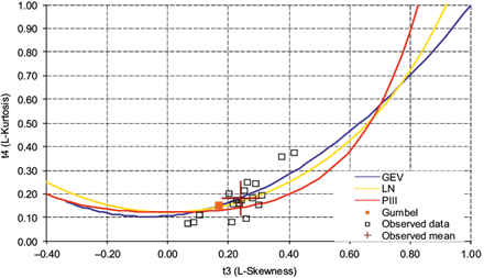
After testing for homogeneity in the three groups, the best model for the fitting of maximum daily precipitations was selected by using the ZDIST statistic as suggested by Hosking and Wallis (1993), 1997). In addition, the L-moments diagram for each of the three groups was plotted in order to choose the most appropriate regional distribution for each group. ZDIST statistic (Table IV) and diagrams (Figs. 3, 4 and 5) show that GEV law represents the best model for annual maximum daily precipitations fitting for the three groups. This result corroborates with the results obtained by the local approach (Habibi et al., 2013; Boucefiane et al., 2014).
4. Regional growth curves and estimates of quantile values
4.1. Design rainfall depth estimation through index-rainfall approach
The regional statistic analysis of maximum daily rainfalls allows drawing regional distribution curves for each group of stations described as being homogeneous in terms of what is shown in Figure 6. Thus, the rainfall index determined for each of the three homogeneous groups is used in Eq. (4) to calculate the maximum daily rainfall for different return periods for the stations that have short observation series, by using the p(F) values of written down in Table V. The main assumption of the rain index method was checked, verifying that the statistic distribution of maximum daily rainfalls in the three homogeneous groups is similar.
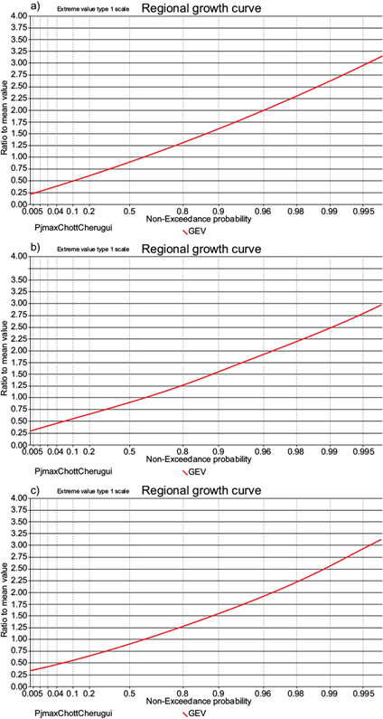
Table V Quantiles for the F function.
| Quantiles function p(F) | Return period (years) | |||||||
| 2 | 5 | 10 | 20 | 50 | 100 | 200 | 500 | |
| Region I | 0.91 | 1.30 | 1.56 | 1.83 | 2.20 | 2.49 | 2.79 | 3.20 |
| Region II | 0.90 | 1.28 | 1.55 | 1.82 | 2.20 | 2.50 | 2.82 | 3.26 |
| Region III | 0.91 | 1.30 | 1.58 | 1.89 | 2.35 | 2.76 | 3.24 | 3.97 |
To calculate the maximum daily rainfall from one of the three groups for a given return period, the average maximum daily rainfall of the series of station i should be multiplied by the corresponding quantile function of Table V using Eq. (9).
This approach will make it possible to estimate rare frequency quantiles in stations with short or incomplete observation series. Also, these quantiles can be calculated for sites without measurement stations by using the maximum average daily rainfall that can be obtained by interpolation.
The estimation of these precipitations frequency is essential to water development and in the design of hydraulic structures. The estimation of quantiles for maximum rainfall is required for calculating flood protection works. The region is subject to repeated floods caused by heavy rainfalls. As an example, the events of October 2011 caused the death of 10 persons and huge material damage in El Bayadh city.
These numbers show the importance of estimating extreme rainfall in development studies and the regional approach as a solution to the lack of rainfall data and the inadequate quality of information measured at some stations.
4.2. Validation of use of regional growth curve for quantiles estimation
Reliability of the regional method for quantile estimation is validated by bias (BIAS) and root mean square error (RMSE) for each return period (Table VI).
Table VI RMSE and bias results of the estimated quantiles.
| T | Bias (%) | RMSE (%) |
| 2 | 13.06 | 14.17 |
| 5 | 13.69 | 14.70 |
| 10 | 13.41 | 15.07 |
| 20 | 13.93 | 17.02 |
| 50 | 14.90 | 21.05 |
| 100 | 15.69 | 24.84 |
| 200 | 16.64 | 29.20 |
| 500 | 18.02 | 35.54 |
| 1000 | 19.40 | 40.84 |
In terms of bias, quantiles estimated from regional information are rather close to those locally estimated. For low return periods (T < 20 years), the bias is practically low. Beyond this threshold, the bias still remains acceptable (< 20%). The root mean square error is below 25% for the quantiles relating to the return periods below 100 yrs.; but, for higher return periods, estimations for daily maximum precipitations should be dealt with caution. These results are comparable to those by Onibon et al. (2005) in Canada, Benhattab et al. (2014) in Algeria, and Malekinezhad and Zare-Garizi (2014) in Iran. Table VII presents the deviations of local estimation to regional estimation of quantiles for the stations of Oued Taria, Mecheria and Ain Skhouna. For T ≤ 10 years, the difference is almost negligible. Beyond this threshold, regional estimate introduces a difference characterized by underestimation or overestimation of quantiles. Ain Skhouna and Oued Taria stations illustrate overestimation. The deviations on large return periods are due to the regional information effect on the estimation of L-CV and L-CS. When the regional estimation of the latters gives values above or below those locally estimated, the regional model tends to overestimate or underestimate the quantiles associated with the large return periods.
Table VII Deviations due to the regional estimation of quantiles.
| Station | Oued Taria | Mecheria | Ain Skhouna | |||||||||
| T (years) | X(T)regional | X(T)local | ERR (%) | X(T) regional | X(T) local | ERR (%) | X(T) regional | X(T) local | ERR (%) | |||
| 2 | 35.3 | 30.8 | 12.7 | 36.22 | 31.07 | 14.2 | 25.0 | 21.5 | 14.0 | |||
| 5 | 50.4 | 42.3 | 16.1 | 51.74 | 45.73 | 11.6 | 35.7 | 33.4 | 6.4 | |||
| 10 | 60.5 | 50.7 | 16.2 | 62.09 | 56.61 | 8.8 | 42.9 | 41.8 | 2.6 | |||
| 20 | 71.0 | 59.3 | 16.5 | 72.83 | 68.04 | 6.6 | 50.3 | 50.3 | 0.0 | |||
| 50 | 85.4 | 71.3 | 16.5 | 87.56 | 84.42 | 3.6 | 60.5 | 62.1 | -2.6 | |||
| 100 | 96.6 | 81.1 | 16.0 | 99.1 | 97.98 | 1.1 | 68.5 | 71.4 | -4.2 | |||
| 200 | 108.3 | 91.5 | 15.5 | 111 | 112.7 | -1.5 | 76.7 | 81.1 | -5.7 | |||
| 500 | 124.2 | 106.4 | 14.3 | 127.4 | 134.1 | -5.3 | 88.0 | 94.8 | -7.7 | |||
| 1000 | 137.1 | 118.5 | 13.6 | 140.5 | 152 | -8.2 | 97.1 | 105.8 | -9.0 | |||
5. Conclusion
The study area is characterized by catastrophic floods like those of October 2011, which caused 10 deaths and significant material damage. The objective of this study is to determine quantiles of maximum precipitation to address a concern: having a better protection against floods through an appropriate dimensioning of structures. Therefore, the regionalization of the annual maximum annual rainfall has highlighted three homogeneous groups in the study area.
The L-moments method made it possible to determine the most suitable probability distribution for the different samples of extreme rainfall, which in this case was the GEV distribution.
It was concluded that extreme precipitations quantiles for a station in one of the three groups and for a given return period, obtained by multiplying the average maximum daily rainfall of the series of this station by the corresponding quantile function extracted from the regional curve, might be estimated reasonably for the study region. This region is prone to repeat disasters caused by floods due to its characteristic heavy downpours. Therefore, this regional approach will be of great interest for hydraulic calculations necessary to design hydrotechnical structures and those for protection against floods. More than 50% of rainfall stations have very short series of observations or series of gaps. Therefore, to overcome this handicap, the results obtained allow estimating precipitations at these stations.

