


 nueva página del texto (beta)
 Inglés (pdf)
 Artículo en XML
 Referencias del artículo
 Enviar artículo por email
 Citado por SciELO
  Similares en
SciELO
Similares en
SciELO 
 Permalink
1. Introduction
Processes and activities involving combustion such as transportation, power plants and industrial activities emit a large scale of atmospheric pollutants. Motor vehicle traffic is the main contributor to road traffic emissions in the ambient air. Appropriate indicators of this environmental burden are nitrogen oxides. Due to human activities, about 40% of the total NOx emissions are released from road activities, 25% from power plants and the rest from other anthropogenic industrial and commercial processes (EEA, 2014). NOx are a group of criteria air pollutants that express the total sum of NO and NO2 (Leighton, 1961; Atkinson, 2000).
NOx do not directly influence the Earth’s radiative balance (Prather, 2001). However, they are catalysts of tropospheric O3 formation (Sjödin et al., 1994; Manahan and Manahan, 2009; Seinfeld and Pandis, 2016), major components of photochemical smog and partly responsible for the creation of acid rain (Chang and Suzio, 1995; Atkinson, 2000; Menz and Seip, 2004). Produced by nitrogen and oxygen at high temperatures, NO and NO2 are highly reactive gases. NO is predominantly emitted from the exhaust systems of the combustion engines (Seinfeld and Pandis, 2016). However, NO in the atmosphere during a short time is oxidized to NO2 (Nielsen et al., 1996; Carslaw and Beevers, 2005). The ratio of NO and NO2 concentrations across highways is defined by many factors such as ozone concentration levels, concentration of fine aerosol particles in the air (Sjödin et al., 1994; Ollinger et al., 2002; Pirjola et al., 2006; Beckerman et al., 2008), road distance (Chen et al., 2003; Costabile and Allegrini, 2007; Gilbert et al., 2007; Wang et al., 2011; Pattinson et al., 2014; Sayegh et al., 2016), and catalyst-equipped vehicles with advanced emission control technologies assistance (Sawyer et al., 2000; Wang et al., 2012), among others.
NOx play a substantial role in the Earth’s atmosphere due to their detrimental effect. In the vicinity of motorways, NOx concentration levels may exceed the ambient air quality guidelines and thus have harmful effects on the environment and human health (Brunekreef and Holgate, 2002). As a result of the fast transformation of NO to NO2, harmful effects are usually attributed to the presence of the later (Last et al., 1994). Average measured NO2 concentration levels depend on meteorological conditions and wind direction but mostly on the distance of the measurement site from highways (Lippmann, 1989; WHO, 2000; Gilbert et al., 2003; Kim and Guldmann, 2011).
The estimation of vehicle emissions has become a notable discussion in the last decades due to the continuous growth of vehicle transportation and its increasing demand. Therefore, numerous emission models have been established for traffic emissions assessment. Emission models are used to estimate pollutant emission levels by calculating road traffic emissions. Emission models are based on the implementation of different parameters, i.e. vehicle and fuel types, driving patterns, fuel consumption, etc., in order to provide emission factors (EFs), which express the emitted mass of a pollutants per driven distance and amount of fuel or energy consumed (Borge et al., 2012; Franco et al., 2013). Vehicle categories and characteristics, emission control technology implementation, operating conditions and fuel consumption are crucial parameters for EFs determination (Smit et al., 2010). There are different models that make possible EFs calculation. Depending on the model the parameters required to determine EFs can be traffic scenario, average traveling speed, second-by-second vehicle data to derive emission information for the complete driving profile or second-by-second vehicle activity parameters of engine power determination (Scora and Barth, 2006; Hausberger et al., 2009; Franco et al., 2013).
In the last few decades, a series of mathematical modeling programs for traffic-related pollutants emissions were established. The first models were created with the initiative of the US Environmental Protection Agency (US-EPA) starting with the primary model AP-42 Compilation of Air Pollutant Emission Factors, published by EPA in 1972. This model compiled emission factors for more than 200 air pollution source categories, including road transport. Subsequently a specialized MOBILE vehicle emission factor model was created considering three primary exhaust pollutants (HC, CO and NOx), different vehicle categories (passenger cars, trucks, buses and motorcycles) that use gasoline, diesel or natural gas for combustion, for the years starting from 1952 to 2050. The MOBILE model was gradually expanded until the year 2010 to MOBILE6.2. Afterwards, the MOBILE 6.2 model was replaced by the MOVES (Motor Vehicle Emission Simulator) model as the EPA’s official emissions model (US-EPA, 2010, 2016). Since then, a number of similar emission inventory programs such as EMFAC, CMEM, originated in the US and Canada, have been created (Scora and Barth, 2006; Barth et al., 2014; US-EPA, 2015).
Numerous emission models were created in Europe for the estimation of pollutants emissions. Most of these models are based on the Gaussian air pollutant dispersion model in the vicinity of linear emitters (Kukkonen et al., 2001). From these models, the mathematical model Handbook of Emission Factors for Road Transport (HBEFA) stands out distinctly. The model was originally developed upon an initial collaboration between the German, Swiss and Austrian agencies for environmental protection. Subsequently, similar agencies from Sweden, Norway and the Joint Research Centre of the European Commission supported the HBEFA. The first HBEFA model (v. 1.1) was published in 1995, providing average emission factors for Germany and Switzerland. From the year 2010, the updated HBEFA 3.1 model provided data for Germany, Switzerland, Austria, Sweden and Norway. The currently available version from June 2014, is HBEFA 3.2. In addition to the previous countries, this model includes also emission factors for France (Keller and Wüthrich, 2014). The HBEFA emissions model was developed based on results of exhaust gas measurements with dynamometric tests of light-duty vehicles (LDV) and heavy-duty vehicles (HDV), including also dynamometric test measurements of LDV and HDV vehicles from real world driving patterns. These procedures made possible to obtain results that correspond to realistic traffic scenarios with the highest possible degree of accuracy.
Within the project of the Ministry of the Environment of the Czech Republic (MŽP ČR VaV/740/3/00) an authorial team from the University of Chemistry and Technology of Prague, ATEM and DINPROJEKT, created the MEFA v.02 model program (ENVIS, 2009). The currently improved version was developed in 2013 and is available as MEFA 13. This model was assembled using already acquired and verified vehicle emissions data of tests performed in the European Union countries, primarily the application of the aforementioned HBEFA model (Skácel and Tekáč, 2014). These data were supplemented using the results of specific emission tests for the characteristic vehicle fleet of the Czech Republic.
Despite the successful development of the mathematical models for road traffic emissions, the calculated results obtained by the application of EFs and the measurement results of the actual concentration of traffic pollutants cannot be considered as identical, which has been confirmed by several studies that performed measurements with minimal influence of external environmental factors (i.e., meteorological conditions could be left out). For this purpose, road tunnels are very suitable.
Tunnel studies were performed in the Van Nuys tunnel in California to verify the models MOVES2010a, MOBILE6.2, and EMFAC2007 (Fujita et al., 2012); the Gubrist tunnel in Switzerland, to verify the HBEFA2.1 model (John et al., 1999; Colberg et al., 2005a); and the Plabutsch tunnel in Austria, to verify the HBEFA1.2 model (Hausberger et al., 2003; Colberg et al., 2005a). The study in the Van Nuys tunnel, based on the comparison of three models, resulted with higher calculated NOx emission factors than the measured NOx EFs from the tunnel experiment (Fujita et al., 2012). The results obtained by using each model differed considerably. However, the measured NOx EFs corresponded the most with MOBILE6.2 model EFs and least with EMFAC2007 EFs (Fujita et al., 2012). In addition, an overestimation of NOx emission factors from HBEFA2.1 (over 50% for LDV and 15% for HDV) was obtained in the study of the Gubrist tunnel (Colberg et al., 2005b). However, in the study of the Plabutsch tunnel, the modeled NOx emission factors for HDV were significantly underestimated compared to the measured results (Hausberger et al., 2003). These facts led to a series of verification measurements carried out in a very short tunnel in the Czech Republic, whose main objective was the validation of a mathematical model for the estimation of real road traffic emissions.
2. Experiment
2.1 Sampling site
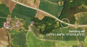
The measurements of NOx emissions were performed in Zeleny most (short tunnel), which is depicted in figure 1. This tunnel is located on Highway D11 in the Pardubice region, approximately 72 km east of Prague. Zeleny most is single-bore tunnel with two lanes of traffic in each direction, a length of 77 m and a cross area of approximately 350 m2 (Fig. 2).
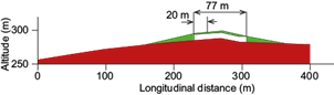
This section of the D11 highway, where high traffic intensity occurs, was put into operation in 2006. The road average inclination in the tunnel section is much less than 1%, hence close to zero.
The sampling site choice was conditioned by the need to ensure stable conditions for air sampling. Ideal sampling sites are long road tunnels without active ventilation. The tunnel environment has special characteristics preserving inner air composition due to limited air circulation. The main advantage of road-tunnel studies is that the conditions are well defined and meteorological effects are excluded. Therefore, measurements of emission levels can be obtained under relatively controlled conditions.
2.2 Measuring system and methods
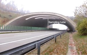
The measurements of NOx concentrations were carried out using a Horiba AP-360 series air pollution monitoring system. The APNA-360 NOx analyzers are based on the chemiluminescence principle with a low detection limit expressed by a volume fraction of 0.5 × 10⁻⁹ (Kato and Yoneda, 1997). The nitrogen oxide analyzer uses a multi-flow modulation method that enables synchronic and separate measurements of NO, NOx, and NO2. NO2 is determined by subtracting NO from NOx (Kato and Yoneda, 1997). The analyzers were calibrated by an accredited calibration laboratory in the Czech Republic. The sampled air was drawn to the analyzer through a probe and a PTFE (polytetrafluoroethylene) sampling tube, which was equipped with an inlet filter and was positioned in the middle of the road tunnel (Fig. 3).
Another part of the measurement consisted in counting the vehicles passing the tunnel section. The assessment of the number of passing vehicles was performed by simple counting. Motor vehicles were divided into two categories: light vehicles (cars and vans with a length up to 6 m) and heavy-duty vehicles (trucks and buses).
The sampling time was divided in 9 min intervals comprised of 3 min average values of NOx. The speed of the vehicles was controlled by calculations and was overwhelmingly equal to the speed limits specified for the measured section of the D11 highway, i.e., 130 km/h for light vehicles (LV) and 100 km/h for heavy-duty vehicles (HDV). Vehicle speeds during each measurement campaign were controlled and maintained at all meteorological conditions.
2.3 Modeling of emission factors for NOx tunnel measurements
To obtain the EFs from tunnel measurements, the HBEFA 3.1 model was implemented. HBEFA 3.1 is a collective of older and new measurements aggregated in an improved model that has access to all existing data.
To specify the traffic scenario, selected parameters of HBEFA 3.1 were used together with the values listed in Table I. The fleet composition of the passing vehicle proceeds from the PHEM model based on summation of vehicles registered in the countries involved in the HBEFA model setup for the selected years (Hausberger et al., 2009). The fleet parameter "business-as-usual" (BAU) D corresponds to the composition of the vehicle fleet registered in Germany. The BAU D fleet composition parameter was chosen to verify the fleet model in the Czech Republic. This choice acknowledges the fact that the great majority of motor vehicles passing through Czech highways are equipped with the same engines as the vehicle engines in Germany. This assumption applies particularly for the most frequently used Czech vehicle brand, i.e. Škoda.
Table I Selection of parameters for a specific road traffic case.
| Selected parameters | Requested values |
| Vehicle categories | Passenger cars (lv) Heavy-duty vehicles (hv + buses) |
| Area of traffic communication | Rural |
| Level of traffic service | Free flow |
| Speed limit | 130 km/h (LV) |
| 100 km/h (HV+Buses) | |
| Road slope gradient | 0% |
| Fleet composition | "BAU" D |
| Selection of years | 2005, 2010, 2015 |
| Pollutants | NOx |
2.4 Data processing
It is very convenient to apply statistical data processing to tunnel measurements. The experimental results were processed using analysis of variance (ANOVA), which is a method used to test the equality of two or more population means by analyzing the variance of taken samples (Massart et al., 1988). This method makes possible to determine whether the differences between samples are due to either random or systematic errors (Dohnal, 2008). Systematic errors cause the mean in one group to differ from the mean in another. ANOVA is usually used to compare the equality of two or more means (Dohnal, 2008).
3. Results and discussion
3.1 Measurement campaigns and sampling point
The study was based on short-term daily measurements performed during the years 2015-2018. A total of six successfully completed measurement campaigns, each lasting at least 2 h, were carried out in different weekdays at different hours during the course of the day. The measurements were accomplished under different meteorological conditions and various traffic situations in order to cover the typical traffic condition in the monitored D11 section. Mean wind velocity was below 5 m s-1 during all measurement campaigns.
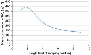
During each of the campaigns, NOx concentrations were measured at different heights in the tunnel to specify the sampling point position. The representative sampling point was chosen on the position where the highest concentration of NOx was detected. The NOx mass concentration dependence on different height positions of the sampling tube is shown in Fig. 4. The sampling point was chosen to be situated at 2 m above the tunnel ground level in the point where the highest NOx concentration was found, as depicted in Fig. 4, for the measurement campaign held on April 13, 2018.
3.2 Time series of the measurement results
Time series of the concentration progress from the monitored compounds NO, NO2 and their sum NOx, were obtained. In figure 5, a typical course of these time series is shown:
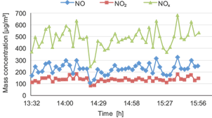
Fig. 5 Temporal variation of the NO, NO2 and NOx mass concentration progress (Zeleny most, April 13, 2018).
The pattern shows that concentrations of NO, NO2 and NOx varied during the whole measurement campaign. The actual hourly mass concentration limit of NOx at standard conditions (20 °C, 101.325 kPa) is 200 µg m-3 (Czech Republic, 2012). In this context it should be mentioned that during the measuring campaign no time interval was recorded in which the actual NOx mass concentration felt below the hourly NOx limit.
For the verification of the impact of other NOx emission sources in the vicinity of the measuring site, measurements of background NO, NO2 and NOx concentrations were performed. The sampling site was chosen to be at a distance of about 100 m eastward of the tunnel portal. The resulting values were almost stable and the mean mass background concentration of NO, NO2 and NOx were 21.3, 44.8, and 82.4 µg m-3, respectively.
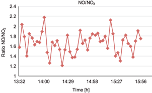
The time series of the ratio of NO and NO2 mass concentrations observed during all the measurement campaigns were found to be very similar. A typical example of this time series is depicted in figure 6.
The time series of the number of vehicles (divided into two categories, LV and HDV) passing through the tunnel section were used to assess traffic intensity. The typical course of traffic operations is shown in figure 7.
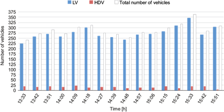
Fig. 7 Total number of vehicles from all categories during the 9-min measurement intervals (Zeleny most, April 13, 2018).
The measurement campaign held on April 13, 2018 lasted about 3 h in which high traffic intensity was noticed. The total number of vehicles that passed through the tunnel section of the D11 highway was 4615. It should be mentioned that during the course of the measuring campaign no time intervals were recorded in which the frequency of LVs felt below 240 crossings. The frequency of HDVs did not fall below five crossings but on the other hand it did not exceed 24 crossings in each 9 min interval.
3.3 Correlation of NOx mass concentration and traffic intensity
An important part of this study was the characterization of the impact of traffic intensity on NOx concentration levels in the short tunnel Zeleny most. During the measurements, simultaneous data of time-resolved NOx concentrations and passing vehicles calculations were acquired. For the statistical assessment of the correlation of the NOx mass concentration generated in the tunnel space and the traffic intensity, analysis of variance was used. Both correlations are graphically expressed in figures 8-10.
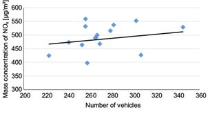
Fig. 8 Correlation of NOx mass concentration dependence and number of passing light vehicles in 9-min intervals (Zeleny most, April 13, 2018).
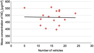
Fig. 9 Correlation of NOx mass concentration dependence and number of passing heavy-duty vehicles in 9-min intervals (Zeleny most, April 13, 2018).
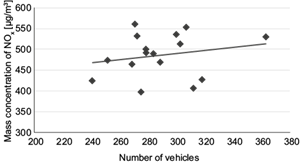
Fig. 10 Correlation of NOx mass concentration dependence and number of passing light and heavy-duty vehicles in 9-min intervals (Zeleny most, April 13, 2018).
The dependence of the NOx mass concentration on the number of passing vehicles of different categories (LV, HDV, total number of passing vehicles) was determined. ANOVA compares whether or not the controlled factor has a significant effect (Massart et al., 1988), so it was used to compare whether the number of passing vehicles had a significant effect on the NOx mass concentration progress, i.e., a measure of linearity. The interpretation of ANOVA is based on the value of the F-test. The linearity test is done by calculating the F-value and comparing it with the tabulated critical F-test value for a given number of degrees of freedom. The results obtained by ANOVA for the example case (April 13, 2018) are depicted in Table II.
Table II Analysis of variance for example case (Zeleny most, April 13, 2018).
| Characteristics of 3-min intervals | Fcalc | Fcrit | |
| Compounds of interest | Vehicle category | ||
| NO | LV | 1.128 | 2.02 |
| HDV | 1.128 | ||
| Total vehicle sum | 1.131 | ||
| NO2 | LV | 1.528 | |
| HDV | 1.705 | ||
| Total vehicle sum | 1.501 | ||
| NOx | LV | 1.227 | |
| HDV | 1.283 | ||
| Total vehicle sum | 1.228 | ||
In the case of the LV category, the results of all measuring campaigns showed a linear dependency of the mass concentration of NO, NO2, and NOx on the number of passing vehicles. In the case of HVs, the linear dependence of the mass concentration of NO, NO2, and NOx on the number of passing vehicles was not ascertained in all campaigns. The results for HDVs were statistically influenced by the infrequent number of all individual vehicles compared to the number of LVs, which significantly influenced the value of random variations for this statistic interpretation.
3.4 Verification of the HBEFA 3.1 model
The road case of the tunnel section in the D11 highway corresponds to the selection of parameters in HBEFA 3.1. Therefore, this mathematical program was applied to the calculation of the emission factors. The mass of NO and NO2 (expressed summarily as NOx), corresponding to LVs intensity, monitored and calculated in the tunnel environment, is depicted in figure11. Additionally, figure 11 depicts the NOx masses calculated by the HBEFA 3.1 model for passing LVs, corresponding to the fleet structures registered in 2005, 2010, and 2015 in Germany. The results show a significant overestimation of NOx emissions calculated by the applied model.
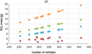
Fig. 11 Comparison of the measured NOx mass in each sampling period with the calculated NOx mass EFs from HBEFA 3.1 for LVs (Zeleny most, April 13, 2018). Red dots: measured NOx mass. Blue dots: NOx mass calculated with EF for 2005. Green dots: NOx mass calculated with EF for 2010. Orange dots: NOx mass calculated with EF for 2015.
NO and NO2 masses, expressed summarily as NOx, corresponding to the HDVs intensity, monitored and calculated in the tunnel environment, are depicted in figure 12. Additionally, figure 12 depicts NOx masses calculated by the HBEFA 3.1 model for passing HDVs, corresponding to the fleet structure of this category registered in 2005, 2010, and 2015 in Germany. The results in figure 12 overestimate NOx emissions calculated by the applied model for the fleet structure of 2005, and underestimate the fleet structure of 2010 and 2015.
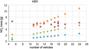
Fig. 12 Comparison of the measured NOx mass by sampling period with the calculated NOx mass EFs from HBEFA 3.1 for heavy-duty vehicles (Zeleny most, April 13, 2018). Red dots: measured NOx mass. Orange dots: NOx mass calculated from EF for 2005. Green dots: NOx mass calculated from EF for 2010. Blue dots: NOx mass calculated from EF for 2015.
4. Conclusions
Measurements of NOx concentration levels were performed in the road tunnel Zeleny most, Czech Republic, in order to verify the impact of traffic intensity and to compare the measured tunnel data with EFs calculated from a comprehensive road traffic emission model. The simultaneous measurement of NOx mass concentrations and the count of passing LVs showed a positive linear correlation between the two variables with a correlation coefficient of 0.321. The simultaneous measurement of NOx mass concentrations and the count of passing HDVs showed a slightly negative linear correlation between the two variables with a correlation coefficient of -0.02. This result may be due to the piston effect generated by the relatively large HDV cross-section passing at high speed through the short tunnel. The results derived from the measurement campaigns were compared to the EFs calculated by the HBEFA 3.1 model for the tunnel case conditions of this study. The results showed an overestimation of NOx emissions calculated using EFs for thr years 2005, 2010, and 2015 with the HBEFA 3.1 model for LVs. The measured NOx emissions are in agreement with the calculated NOx emissions using EF for HDVs in 2005. A considerable underestimation of NOx emissions calculated from EFs for the years 2010 and 2015 was found for HDVs. This outcome is emphasized by the fact that, despite all similarities in the fleet composition between the Czech Republic and Germany (section 2.3, Modeling of emission factors for NOx tunnel measurements), it can be assumed that the vehicle fleet monitored in the Zeleny most section of the D11 highway consists of slightly older vehicles with less rigorous emission standards than the fleet in Germany. Another fact that can be mentioned regarding the contribution of NOx emissions in the tunnel environment, is that HDVs make up only a small part of the total number of vehicles observed in all measurement campaigns (Fig. 7).
The results of the verification measurements carried out in a very short tunnel in the Czech Republic corresponded to the results obtained in other tunnel studies performed under various tunnel conditions and structures (length, non/passive ventilations, single/dual tube structure, different numbers of road lines, different road gradients, etc.). An overestimation of modeled emission factors for road traffic NOx emissions has been pointed out in previous works and was confirmed by the results in this work. Further studies are needed in the future on this topic.

