1. Introduction

The southern part of the Gulf of California, located between the eastern tip of the semiarid Baja California peninsula and the mainland coast on northwestern Mexico, is the region where water exchange and forcing associated with the Pacific Ocean produce a different climate than in any other part of the Gulf of California (^{Velasco-Fuentes, 2003}). This difference in climate generates one of the main mechanisms for the fertilization of this region (^{Álvares-Borrego, 2012}), which is associated to the development of mesoscale structures such as eddies, jets and meanders (^{Salinas-González et al., 2003}), circulation features that transfer important properties from one coast to another (^{Figueroa and Robles, 1989}). Because most of the year the southwestern Gulf of California remains cloud free, this region is ideal for using satellite images to study and observe the development and presence of these mesoscale structures (^{Pegau et al., 2002}).

The Bay of La Paz (BLPZ), located on the southwestern coast of the Gulf of California (GC) 180 km from the mouth (Fig. 1), is considered the largest bay in the Gulf of California (^{Sánchez-Velasco et al., 2004b}). This region is also characterized by strong seasonal variability, high diversity and abundance of fish species and as a spawning area for many species of great ecological significance (^{Sánchez-Velasco et al., 2006}) with an important presence of marine mammal populations, such as whales and dolphins. The BLPZ is bounded on the east by the insular region of the archipelago Espíritu Santo, designated by UNESCO as a protected wildlife area; on the north by San José Island and the North Mouth, where the main interaction with the GC occurs; on the southern part by the city and port of La Paz, the main urban area in the region with a population of ~ 290 000 inhabitants (^{INEGI, 2015}); and on the northwest by the sierra El Mechudo, a mountainous region of difficult access, wide altitudinal gradient (> 800 m) and several mountain passes where northwestern winds cross the peninsula, modifying their characteristics before interacting with the bay during winter-spring season.

Fig. 1 Geographic location and bathymetry characteristics of the Bay of La Paz 

Figure 2 shows an example of the strong exchange of properties between the BLPZ and the GC (mainly through the North Mouth) using weekly composites of sea surface temperature (SST) and surface Chlorophyll a concentration(Chl-a) satellite images (NOAA-Pathfinder project and MODIS-Aqua sensor). SST has been used as an indicator of the processes that generate changes in Chl-a, which has a direct relationship with the water column structure (^{García-Gorriz and Carr, 1999}). A well-mixed water column facilitates the fertilization process while a stratified one inhibits fertilization of the upper layer (^{Reyes-Salinas et al., 2003}) although primary productivity and Chl-a (estimated via natural flourescence and satellite images) have been used to analyze the interaction between mesoscale structures and distribution of ocean productivity and phytoplankton (^{Chelton et al., 2011}). ^{Coria-Monter et al. (2014)} observed the differential distribution of diatoms and dinoflagellates in the presence of a cyclonic eddy confined in the BLPZ.

Fig. 2 Satellite images of weekly composites showing the exchange of properties between the BLPZ and GC: (a) Sea surface temperature (NOAA-AVHRR Pathfinder project, 21 November 1999) and (b) chlorophyll a (MODIS-Aqua, 06 November 2004). 

The hydrographic conditions in the BLPZ are influenced by three main factors during an annual cycle: (1) hydrographic variability in the southern GC; (2) high solar radiation (high evaporation rates); and (3) local wind forcing: strong northwesterly winds during winter and early spring with values ~ 8 to 12 m s^-1 and the onset and intensity of the North American Monsoon with moderate south and southeastern winds with magnitudes ~ 4 m s^-1 in summer and early fall (^{Marinone et al., 2004}; ^{Turrent and Zaitsev, 2014}). This wind pattern, jointly with the coastal orientation and the orographic continental effect on BLPZ, could generate advection and coastal currents in winter and cyclonic surface circulation throughout summer and early fall (^{Jiménez-Illescas et al., 1997}; ^{Sánchez-Velasco et al., 2006}; ^{Coria-Monter et al., 2014}).

These surface circulation characteristics, along with the environmental conditions and physical processes (turbulent mixing, gyres and filaments), can enhance primary production and organic matter export, impacting local upwelling events and phytoplankton populations (^{Bibby et al., 2008}). These relationships between the biological and environmental factors observed in the bay have demonstrated strong physical-biological coupling. The local seasonal wind pattern could be forcing changes in the SST, upwelling processes and mesoscale variability. The hypothesis of the generation of biological enrichment events in the BLPZ by the action of the wind annual cycle in the form of wind stress curl is resumed in this work. Our main objective was to determine the annual and semi-annual components of the seasonal cycle of SST and Chl-a for the BLPZ using a harmonic fit and empirical orthogonal function decomposition, and then relate them to temporal and spatial variability of wind stress curl. An additional goal of this paper was to describe the relationships between the high biological productivity (represented by the Chl-a variability patterns) and wind stress curl at a seasonal scale (winter-summer).

2. Data and methods

The data used in this analysis were monthly composites of SST and Chl-a satellite EOS-PM-1 MODIS-Aqua (http://modis.gsfc.nasa.gov/) http://modis.gsfc.nasa.gov/ with a 4 × 4 km pixel array covering the period from July 2002 to December 2013. The monthly mean ocean surface wind data were obtained from the Cross-Calibrated Multi-Platform (CCMP) project (https://podaac.jpl.nasa.gov/) for the period from January 2002 to December 2011 at a horizontal resolution of 0.25º × 0.25º covering the southern part of the GC (22-25.5º N, 108-111º W) and re-binned into 4 × 4 km to produce the same spatial resolution used in both SST and Chl-a. The study was undertaken in the BLPZ located on the western coast of the GC (24-25º N, 110-111º W; Fig. 1). Monthly climatological fields of each variable (SST, Chl-a and ocean surface wind) were calculated by averaging each month for the periods 2002-2013 and 2002-2011, respectively and ordered in arrays of 12 monthly climatological data average T (x, t) where x represents the number of cells or pixels of each image and t represents the number of months of the climate cycle as follows:

(1)

where t _i , represented the ith climatological monthly mean. In this case, we used this data array in a harmonic analysis to investigate their fit to a seasonal cycle composed of annual and semi-annual harmonics plus mean values as follows:

(2)

where A ₀ was the annual mean, A ₁ , w ₁ , and φ₁ were amplitude, frequency, and phase of the annual signal and A ₂ , w ₂ , and φ₂ were the corresponding to the semi-annual signal. Most commonly, parameters of the seasonal cycle (amplitudes and phases) have been obtained by least square fitting of Eq. (2) to climatological monthly means.

Alternatively, a derivation of conventional empirical orthogonal function (EOF) analysis called “spatial variance EOF” or “gradient EOFs” (^{Lagerloef and Bernstein, 1988}; ^{Palacios, 2004}) could be computed after removing the spatial mean at each time step to decompose gradients of spatial variability rather than temporal variability of the parameter itself (^{Kelly, 1998}). The resulting anomalies or ‘residual’ matrix data sets (the adjusted monthly climatologies) were used in the EOF analysis to identify the main modes of SST and Chl-a spatial variance with equivalent eigenvalue solutions that decomposed modes ranked by their spatial variance (^{Lagerloef and Bernstein, 1988}). This EOFs traditional method variation was used when we required to analyze the variance associated with characteristics that did not vary much over time, such as strong horizontal gradients, fronts, thermal gradients, upwelling fronts and the same annual cycle (^{Paden et al., 1991}).

The wind stress components (N m^-2) and wind stress curl (N m^-3) were estimated by the method described in ^{Large and Pond (1981)} and modified by ^{Trenberth et al. (1990)}, using the equation τ = (τ_x, τ_y) = ρC_D|V|(u, v) where τ is the wind stress and τ_x, τ_y its zonal and meridional components; ρ is the density of air; C _D is the drag coefficient; V is the velocity vector, and |V| its magnitude. Wind stress curl is indicative of smaller-scale dynamics associated with coastal upwelling, inducing an offshore mass flux in the upper ocean that is compensated near the coast by vertical flux of nutrient-rich, colder waters from below the source (^{Milliff and Morzel, 2001}). Finally, the correlation patterns were computed at each point between SST-Chl-a adjusted monthly climatologies and wind stress curl climatic series (January-December) by means of linear regression analysis (LRA).

3. Results

Figure 3 shows the largest seasonal fluctuations represented by the standard deviation (SD) variability computed from each monthly time series of the satellite-derived observations in the BLPZ (time-average SST [x, t̃], Chl-a [x, t̃] and surface wind velocity [x, t̃] values). The SD SST pattern had differences of ~ 1 ºC with respect to the GC whereas the SD Chl-a pattern showed the largest seasonal fluctuations and maximum variability values along the coast, mainly south and northern coasts (> 1 mg m^-3). Both parameters showed an out-of-phase behavior with respect to the GC. The SD surface wind velocity pattern (Fig. 3c) showed a large gradient perpendicular to the coast with maximum values along the northern coast (> 1 m s^-1) despite the low resolution in the original CCMP images. The bottom panels represented the time plot (space-average) of the annual cycle of SST, Chl-a and wind speed; all averages exhibited a clear seasonality with minimum SST values in February (22.3 ºC) and maximum during September (31.4 ºC). The Chl-a time series depicted a semi-annual cycle with a first larger peak occurring in winter (1.8 mg m^-3) and a second one during spring-summer (1.4 mg m^-3). The annual cycle of wind speed showed high values during the winter period (> 2 m s^-1) and minimum values during summer (< 1 m s^-1). These patterns reflect the basic seasonal average geography of the BLPZ climate system and can be used as initial conditions in numerical models and to derive estimates of heat storage or surface conditions.

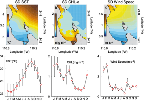
Fig. 3 Surface plots of standard deviation (SD) variability (time-averaged) of MODIS-Aqua satellite-derived. (a) Sea surface temperature (SST), (b) chlorophyll a (Chl-a) and (c) cross-calibrate multi-plataform (CCMP) wind speed for the Bay of La Paz region (24-25º N, 110-111º W). The curves on the lower side correspond to the average seasonal cycle for each variable. Observed averages (red circles) and vertical bars indicate one standard deviation. 

Figure 4 shows the spatial anomalies averaged over the four seasons of (a) SST and (b) Chl-a after removing the spatial mean at each time step showed in Figure 3 (bottom panels). Winter SST anomalies showed a strong north-south thermal gradient located between the BLPZ and the GC with positive values (0.2-0.5 ºC) in the central and southern part of the BLPZ while the winter Chl-a anomalies showed a higher concentration of positive values along the western coast (0.5-1.0 mg m^-3). In spring, an intrusion of SST negative anomalies appeared next to the northern coast and deep zone while Chl-a continued to show high positive values (0.2-0.5 mg m^-3) in the northern and southern coast of the bay. By summer SST showed the inverse pattern of winter, negative anomalies (-0.4 to -0.8 ºC) in the southern coast and along the bay whereas Chl-a showed a reinforcement of high positive values (0.2-1.0 mg m^-3) next to the southern coast and center of the bay. By autumn both SST and Chl-a anomalies showed a relaxation in the values of positive and negative anomalies. The thermal differences observed during winter and summer anomalies showed that surface waters of the bay are less cold (warm) than the GC during an annual cycle.

Fig. 4 Seasonal anomalies calculated after removing the spatial mean at each time step of (a) SST and (b) Chl-a; winter: DEF, spring: MAM, summer: JJA and autumn: SON based on 11 complete years, 2002-2013. 

Figure 5 shows the results of the harmonic fit applied to the SST, Chl-a and wind stress curl monthly climatologies, respectively (annual and semi-annual amplitudes, together with the percentage of the variance explained by the fit). The harmonic fit explains a large percentage of monthly variability throughout much of the bay with R² range of 99% for SST, > 50% for Chl-a, and > 20% for wind stress curl (Fig. 5g, h, i). In Chl-a, the contribution and dominance of the seasonal cycle (Fig. 3, bottom panels) was observed mainly in the vicinity of the GC and central part of the bay whereas in the southern coastal region it showed values ~ 30%. In the wind stress curl, the contribution of the seasonal cycle was observed mainly in the coastal shallow area (southern part of the bay).Two particular features in the SST annual amplitude (Fig. 5a) were the cooling and warming patterns in all the bay with amplitudes of ~ 4 ºC and the gradient or front with direction northwest-southeast that delimited the high amplitude values (> 5 ºC) in the vicinity of GC. The Chl-a annual amplitude (Fig. 5b) recorded high values (> 0.6 mg m^-3) along the northern and southern coasts delimited by topography (indicated by the 200-300 m depth contours). The wind stress curl annual amplitude (Fig. 5c) showed high values only in the southern part of the BLPZ (> 0.08 N m^-3). The semi-annual amplitude of SST (Fig. 5d) had a reverse pattern from the annual amplitude; the highest values were observed in the southern coast of the BLPZ (> 1 ºC) whereas in both Chl-a and Curl (Fig. 5e, f) the semi-annual constituents were similar to those of the annual amplitudes. This suggests that both are highly variable on an intraseasonal scale (values of > 0.5 mg m^-3 and > 0.05 N m^-3, respectively) in areas of high nutrient concentration, mainly along the southern coast and bounded by the 200-300 m depth contours.

Fig. 5 Harmonic fit: Annual amplitude constituents for (a, b, c) SST (ºC); Chl-a (mg m^-3) and wind stress curl (N m^-3), respectively; (d, e, f) semi-annual amplitude constituents for the same variables; and (g, h, i) percentage of explained variance by the harmonic fit for the same variables. Contours indicate the 200 and 300-m isobaths. 

The features observed in the SST and Chl-a annual amplitude patterns were best explained in terms of the annual phase (Fig. 6a, b) defined as a time span (in months, positive or negative) between the beginning of the year (relative to January) and the first peak of the cycle. The annual phase values indicated a sharp gradient between BLPZ and GC; in both variables the phases showed an important lateral variability, particularly in the southern and central region and differences of one month between the GC and the BLPZ. The phase values varied in the range from 9 to 10 months for SST and from 5 to 6 months for Chl-a. The distribution of annual phase of SST and Chl-a reflected the local circulation characteristics and other sources of annual fluctuations such as local conditions of stratification, air-sea heat exchange and seasonal wind direction reversal in the BLPZ during summer (the monsoonal cycle), generating nutrient-rich water advection to the center of the bay (^{Pardo et al., 2013}). This pattern was consistent with the phenomenon in which the bay showed an average phase lag respect to the GC for about one month in the seasonal cycle of surface water heating and cooling (and its effect on primary productivity). The semi-annual phase constituents in both variables (Fig. 6c, d) were only important in localized areas along the coast; values ranged from two to three months for SST and from one to two months for Chl-a, associated with the strong northwesterly wind forcing that commonly cools the northern coast of the bay during winter (December to February) and increases the presence of nutrient-rich coastal waters.

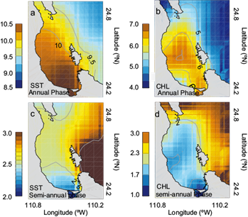
Fig. 6 Harmonic fit: Phases of annual (a, b) and semi-annual (c, d) constituents for SST and Chl-a, respectively, both in months relative to January. 

Figure 7 shows the spatial variance EOF decomposition of the adjusted monthly climatologies (after removing the spatial mean at each time step shown in Fig. 3, SST and Chl-a bottom panels). The EOF₁ of SST (Fig. 7a) explained 92% of the variance, which confirmed that the bay has a different heating and cooling variability of surface waters with respect to the GC. This variability pattern may be influencing seasonal temperature ranges, exerting a slight delay in winter (summer) cooling (warming) between the BLPZ and GC. A strong SST gradient or front associated to water exchange between the bay and the GC through the North Mouth was observed with the zero crossing corresponding to the eastern boundary of the BLPZ and GC. The pool of cooler-than-average water modulation observed in the BLPZ could have been associated with cold water penetration in the surface layer at the beginning of spring and summer (^{Pardo et al., 2013}). The SST EOF₂ pattern (Fig. 7b) explained 6.3% of its spatial variance, a percentage higher than that expressed by the traditional method of EOF temporal variance (not shown) revealing that SST variability in the BLPZ would have been statistically insignificant and obscured in the EOF traditional analysis. This pattern showed the weakening of the gradient observed in the EOF₁ and water exchange between the bay and the GC, similar to that shown from spring SST anomalies (Fig. 4a).

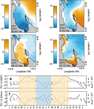
Fig. 7 Surface plots of EOF₁ and EOF₂ calculated after removing the spatial mean at each time step (adjusted monthly climatologies) for: (a, b) SST, (c, d) Chl-a, respectively, and (e, f) time-series data indicate the temporal evolution of the EOF₁ (black line) and EOF₂ (dotted line) for SST and Chl-a, respectively, joint with the average seasonal cycle of wind stress (arrows; N m^-2). Bar in yellow (blue) represents the periods spring-summer (autumn-winter). Time series are repeated twice for clarity. 

The dominant mode in the Chl-a EOF decomposition accounted for 48% of the variance of the adjusted annual cycle (Fig. 7c). Above-average Chl-a concentration occupies much of the bay; high loadings observed in the central part of the BLPZ (deep zone) and along the coast could have been associated to the spatial patterns of the local circulation reported in hydrographic studies during the summer-autumn period within the BLPZ (^{Monreal-Gómez et al., 2001}; ^{Sánchez-Valasco et al., 2006}; ^{Coria-Monther et al., 2014}), providing a strong advection and exchange of high Chl-a concentration between the BLPZ and the GC, mainly through the North Mouth. The EOF₂ of Chl-a (Fig. 7d) explained 31% of the variance; high values were observed mainly along the coast, which suggests upwelling events associated to strong local atmospheric forcing (northwesterly surface wind) could be generating advection and strong coastal currents mainly during the winter period (^{Obeso-Nieblas et al., 2007}). Both patterns were similar to those shown from winter to summer in Chl-a average seasonal anomalies (Fig. 4b) associated with surface enrichment deriving from cold coastal water during these periods. Both modes reflect the regional dynamics of the physical-biological coupling, determined mainly by the local wind forcing pattern, incoming solar radiation, and others.

The time plot of each EOF scores of both variables, jointly with the average seasonal cycle of wind stress vectors (arrows), are shown in Figure 7e, f. The mode 1 amplitudes (black line) confirmed the out-of-phase annual cycles between SST and Chl-a with the positive (negative) peak observed in SST (Chl-a) during spring-summer (yellow bar) and a negative (positive) peak during autumn-winter (blue bar). This last one suggested that both spatial variability patterns were the most intensified during these periods, and their timing was consistent with the average seasonal cycle of wind stress (arrows). The mode 2 amplitudes (dotted lines) depicted negative values occurring between April and July for SST (peak in June) and positive values occurring between November and February (peak in December) for Chl-a. The monthly wind stress annual cycle (magnitude and direction; N m^-2 × 10^-4) showed strong northwesterly wind stress during winter (blue bar) decreasing in intensity during spring and changing southerly during summer (monsoonal cycle). This wind stress annual cycle may have driven anomalous Ekman transport along the year enhancing vigorous currents along the coast, and downwelling during winter that switches to eddy upwelling events during summer (^{Taylor et al., 2008}). The spatial variability patterns and temporal amplitudes of each gradient EOF calculated after removing the spatial mean at each time step of both variables reflected that a significant proportion of this variability may be explained by the regional atmospheric wind forcing pattern.

Since the principal component series for Chl-a were roughly in quadrature with about a two-month phase lag (the sampling errors [not shown] of the first two Chl-a EOF, clearly overlapped [^{North et al., 1982}]), which suggested that a combination of the first two eigenvectors was necessary to describe space-time evolution. In this case, a better alternative to describe the complex space-time feature was to use the extended EOF (EEOF) technique. The details of this analysis were described in ^{Weare and Nansstrom (1976)} and ^{Herrera-Cervantes and Parés-Sierra (1994)}. In this study the Chl-a EEOF analysis used a two-month lag in addition to the simultaneous spatial covariance. Therefore, each of the resulting EEOFs yielded a three-map sequence at months 0, 2 and 4. Since the second eigenmode preceded the first one (not shown) for about two months, we could concatenate the two modes into a single six-map series with the Lag 4 map of EEOF₂ coinciding approximately with the Lag 0 map of the EEOF₁.

Figure 8 shows the first two Chl-a EEOFs, each one consisting of a sequence of three maps (Lag 0, 2, 4). The EEOF₂ (Fig. 8a), showed the most conspicuous feature associated to the presence of high positive variability linking the northern coast of the bay, shifted and extended southward. By Lag 4, high positive variability appeared to become stationary and started to weaken, but the southern high variability pattern began to intensify showing a northward movement covering the central part of the bay. This situation continued at Lag 0 and Lag 2 of EEOF₁ (Fig. 8b). By Lag 4 of EEOF₁, the central high variability began to dissipate. Lag 4 of EEOF₁ was almost a similar image of that at Lag 0 of EEOF₂. Thus a half-cycle of the oscillation took approximately six months. Contours of the wind stress curl (based on over 11 years of data and calculated for winter-spring and summer-autumn periods) were superimposed on the EEOF₂ and EEOF₁, respectively. The sequence interpretation was that positive anomalies of Chl-a variability could only be explained by the effects of the positive curls observed during winter-spring/summer-autumn periods (positive curl inducing upwelling flow).

Fig. 8 Space-time structures of the first and second EEOF of Chl-a for Lag 0, 2 and 4 months. Time increases by two months in successive maps from top to bottom. Contours of the averaged wind stress curl (N m^-3) calculated for: (a) the winter-spring period (December-May) and (b) the summer-autumn period (June-November) and superimposed respectively over the EEOF₂ (left panels) and over the EEOF₁ (right panels). Negative contours are dashed. 

Figure 9 shows the spatial distribution of the correlation coefficients (surface plot of the R values) obtained using the LRA between each SST(x, t) and Chl-a(x, t) adjusted monthly climatologies (spatial anomalies) series and wind stress curl annual cycle. Figure 9a showed the strongest negative correlation between SST and wind stress curl in the blue areas along the northern coast (R = ~ -0.4) and a weak statistical relationship in the southern area, but there are significant similarities to that of the SST-EOF₂ pattern (Fig. 7b). Figure 9b shows the area where Chl-a and wind stress curl strongly co-vary (R > 0.4-0.5, P < 0.05), indicating a better statistical relationship between both parameters. This spatial pattern was closer to the Chl-a-EOF₂ pattern (Fig. 7d), suggesting that at seasonal and semi-annual scale wind stress curl could drive the formation of these patches of high biological enrichment along the coast.

Fig. 9 Surface plots of the correlation coefficients from the linear regression between (a) SST and (b) Chl-a adjusted monthly climatologies series (seasonal anomalies) and wind stress curl annual cycle as the independent variable 

4. Discussion

A relatively high spatial resolution of satellite-derived SST and Chl-a data were useful in delineating the seasonal variability of the quasi-permanent biophysical coupling induced particularly by the regional surface wind stress curl pattern. The results of this study were consistent with those from previous ones (^{Sánchez-Valasco et al., 2006}; ^{Pardo et al., 2013}; ^{Coria-Monther et al., 2014}; ^{Turrent and Zaitsev, 2014}); nonetheless, new details have emerged to our knowledge and understanding of common and unique features of seasonal variability in the ocean-atmospheric system of the BLPZ. Harmonic fit displayed coherent spatial patterns dominated by the seasonal cycle showed in Figure 3 (bottom panels) of warming and cooling of surface waters and their effect on biological productivity; this showed us a view of this biophysical coupling observed along the bay and revealed the extent to which these variables could be affected particularly by diverse forcing, such as regional wind pattern, local income solar radiation, air-sea heat exchange, and others. The first two gradient EOF modes of both variables (computed after removing the spatial mean at each time step) captured the effects of the local wind forcing pattern (mainly over the Chl-a variability). During winter the presence of northwesterly wind conditions could be modulating advection and vigorous coastal currents augmented by Ekman suction offshore whereas during summer, southerly winds associated to seasonal wind direction reversal (monsoonal cycle) could infer the wind-driven offshore Ekman transport. Thermal differences and water exchange with the GC were also consistent with the results.

The amplitude time series (time plot of the EOF₁ and EOF₂ scores; Fig. 7f) of the Chl-a seasonal variability, depicted the bi-modal period of high primary productivity in the BLPZ, a transition from the high values observed along the coastal areas during winter-spring to a redistribution of high primary productivity along the bay during the spring and summer period. Although the Chl-a seasonal variability patterns described by EOF₁ and EOF₂ modes were complex and their amplitude time series had similar schedules (making it difficult to discern seasonal patterns in the time series), high availability of the primary productivity observed in Figure 4b could have been attributed to the timing with the seasonal pattern of wind forcing (Fig. 7f; arrows); during winter, northwesterly wind-driven seasonal upwelling along the coast whereas during summer, southerly wind and mesoscale structures (filaments, meanders, eddies) driven nutrient-rich water advection to the center of the bay. ^{Monreal-Gómez et al. (2001)} attributed the origin of these local mesoscale eddies to wind forcing whereas ^{Coria-Monter et al. (2014)} proposed that these quasi-permanent cyclonic eddies confined in the BLPZ during spring and summer could be responsible for redistribution and transport of high concentrations of nutrients to the euphotic layer, influencing the mixed layer depth.

This timing with the seasonal wind forcing pattern could be better observed using the EEOFS technique; during the winter-spring period, the sequence of Lag 0, 2 and 4 of EEOF₂ (Fig. 8a) appeared to conform very well with the establishment of Chl-a high variability patches over the coast, coinciding with the positive values of the wind stress curl calculated during this period. During the summer-autumn period, positive values of the wind stress curl observed along the bay coincided with high positive variability in the pattern depicted by the sequence of Lag 0, 2 and 4 of the EEOF₁ (Fig. 8b) in the south and center of the bay. Thus during a typical North American monsoon season, high biological enrichment may occur along the BLPZ.

Finally, the spatial distribution of the correlation coefficients between SST and wind stress curl (Fig. 9a) indicates a weak statistical relationship in the southern and central part of the bay (|R| = ~ 0.2), but the high negative correlation values observed in the northern area agree significantly to those of positive wind stress curl superimposed on the EEOF₂ during the winter-spring period (Fig. 8a). The correlation map between Chl-a and wind stress curl (Fig. 9b) showed the area where both parameters strongly co-varied. This area of high positive correlations (R > 0.4, P > 0.05) was similar to that where the Chl-a-EOF₂ and the sequence of Lag 0, 2 and 4 of EEOF₂ scores were > 5.0 (Fig. 7d and Fig. 8b), coinciding with the region with high positive anomalies are observed (Fig. 4b) and where an intense wind-driven winter upwelling and complex summer mesoscale variability has been reported by others authors (^{Pardo et al., 2013}; ^{Coria-Monther et al., 2014}). The different physical-biological responses to wind annual cycle oscillations arise from a combination of ecological and physical dynamics, suggesting that at seasonal scale, the wind stress curl could drive the formation of these patches of high biological enrichment along the BLPZ. Our results emphasize the need for detailed observations on the wind variability in different stages of quasi-permanent physical-biological coupling processes and the mechanisms occurring there.

5. Conclusion

The temporal and spatial resolution of satellite-derived SST and Chl-a data allowed the observation (separately on the two fields) of the physical-biological coupling of very near-shore environments during seasonal processes and their relationship with the wind forcing pattern in the BLPZ. The similarities identified between the distinct annual cycles of SST, Chl-a and wind stress curl in both harmonic fit and gradient EOF analyses could be regulating the intense biological productivity associated to the presence of coastal surface waters rich in nutrients during the winter-spring and summer period; these results support the knowledge that strong coupling between the quasi-permanent patch of cold water and high biological productivity observed in the BLPZ are induced by the seasonal cycle of a regional wind forcing. This study provides a descriptive framework that should be useful to examine the physical-biological coupling processes quantified by these observations. With the recently established marine region of the archipelago Espíritu Santo as protected wildlife area (^{SEMARNAT, 2014}) these results may also be useful to provide valuable information for purposes of sustainability and management of the offshore waters.