


 nova página do texto(beta)
 Inglês (pdf)
 Artigo em XML
 Referências do artigo
 Enviar este artigo por email
 Citado por SciELO
  Similares em
SciELO
Similares em
SciELO 
 Permalink
1. Introduction
Radial velocity of Doppler weather radars is widely used in data assimilation, wind field retrieval, and disaster monitoring. Velocity ambiguity is a common problem in the application of radar velocity fields. Radars obtain the radial velocity of a target by measuring the phase difference between adjacent pulses. The measurement range of velocity is (-V max , + V max ). V max is called Nyquist velocity, and can be expressed as:
 (1)
(1)
where λ is the wavelength and PRF is the pulse repetition frequency. The relationship between true velocity V T and measured velocity V R is:
 (2)
(2)
When |V T | < V max , n = 0 and V T = V R , V R is unambiguous; when |V T | < V max , n ≠ 0 and V T ≠ V R , V R is ambiguous. n is the Nyquist number.
Prior to the application of velocity fields for data assimilation or wind field retrieval, V R must be converted into V T , which is called velocity dealiasing. Velocity dealiasing can be realized through hardware- or software-based methods. The hardware-based approach adopts the staggered-PRT (Doviak and Zrnic, 2006) technology, which can amplify V max many times. However, this method is limited by non-uniform sampling (He et al., 2012) and radar system updating. In addition, velocity ambiguity remains when V T > V max . Therefore, software-based methods (velocity dealiasing algorithms) as an alternative for radar data quality control have been a hot issue in the past decades.
Since the 1970s, many dealiasing algorithms have been developed. In the first 1D dealiasing algorithm, Ray and Ziegler (1977) hypothesized that all velocities in one radial direction were in normal distribution, based on which the ambiguous points were corrected. This algorithm is sensitive to noise and wind shear. In another 1D dealiasing algorithm developed later, Bargen and Brown (1980) assumed that the first point in one radial direction was not ambiguous and not noisy, and then used the average of several points to correct ambiguous points. They also designed an interactive method to further process ambiguous data by manual intervention. This algorithm fails when the first point is noisy or ambiguous. Moreover, the interactive method is not easy to apply. Hennington (1981) put forward a dealiasing algorithm by using external wind fields as reference. This algorithm was not influenced by missing points, noise or wind shear, but an external wind field that matched radar spatial and temporal resolutions was hard to find (James and Houze, 2001). The above three algorithms are simple but weak for dealiasing. Nevertheless, their clues of “point-block” comparison (the reference velocity is obtained from one echo block to judge whether a point is ambiguous) and “point-wind field” comparison (the reference velocity is obtained from external wind field to judge whether a point is ambiguous) are well inherited and extended in later algorithms. Point-block comparison was then extended to 2D, 3D and 4D; the external wind field was replaced by the vertical velocity azimuth display (VAD; Lhermitte and Atlas, 1961; Browning and Wexler, 1968) wind profile, or the wind field output from a numerical model (e.g., Lim and Sun, 2010).
Merritt (1984) proposed the first 2D algorithm. First, a velocity field was divided into several regions that had the same Nyquist number; then the borders of each region were identified; finally, a wind field model was used to process the isolated echo blocks. This algorithm was later modified by adding a monitor to decide whether the wind field model was correct (Boren et al., 1986). Based on Merritt’s algorithm, Bergen and Albers (1988) replaced the wind field model with sounding. They also discussed the influences of noise on the ground clutter region and how to eliminate it. Eilts and Smith (1990) developed a new 2D dealiasing algorithm by combining Bargen and Brown’s and Hennington’s methods. This algorithm searches reference velocity from the points of two adjacent radials and from the VAD wind profile in four steps; then, using this reference, the ambiguous data are corrected. It was modified by He et al. (2012) from four aspects as noise removal, first radial selection, executive order, and error check. It was applied to S-band radars in China. James and Houze (2001) developed a 4D dealiasing method. The elevation angle and time information were added to solve initial ambiguity. The ambiguous points at a low elevation angle could be corrected by referring to those at high elevation angle. Zhang and Wang (2006) also extended the Eilts and Smith’s algorithm to a 2D multi-pass dealiasing algorithm (2DMPDA). This algorithm solved the initial ambiguity by searching the weakest wind region and judging ambiguity by using more radial points.
Yamada and Chong (1999) developed a VAD-based dealiasing algorithm. The initial position of dealiasing was selected to the distance circle with most points, and ambiguity was corrected by referring to VAD wind information. Since ambiguous data could cause error to VAD, a modified VAD (MVAD) was proposed by Tabary et al. (2001). The MVAD utilized the velocity gradient to retrieve vertical wind profiles, thus it reduced influence from ambiguous data. Later, a three-step dealiasing algorithm based on MVAD was proposed by Gong et al. (2003). First, global ambiguous data were corrected by MVAD; then local ambiguous data were restored by VAD; finally, residual ambiguous data were eliminated by using the continuity principle along radial direction. This algorithm was later optimized by Xu et al. (2011).
Jing and Wiener (1993) used transformed dealiasing to solve the extreme values of a linear function. The ambiguous points of one echo block were eliminated by using an environmental wind field. This algorithm was later revised by Witt et al. (2009). Using image recognition technology, a dealiasing algorithm based on zero isodops (lines composed by points whose velocities are close to zero) searching was proposed by Li and Wei (2010). First, zero isodops were identified from 2D images; then the velocity field was divided by zero isodops into positive and negative regions; finally, ambiguous points were corrected by judging whether the sign of a velocity point was consistent with the region it was in.
The general shortcoming of the above dealiasing algorithms is noise suppression. Dealiasing algorithms are all based on the hypothesis that velocity fields are spatially continuous. In case of discontinuity, these algorithms might produce errors. From the perspective of spatial distribution, noise can be divided into two types: isolated noise and continuous noise. If a noisy point is surrounded by more good points (non-noisy points including missing points) than noisy points, it is called an isolated noise; otherwise it is called a continuous noise. For example, in a 3 × 3 window in Figure 1, Ns is surrounded by six good points and two noisy points, so it is an isolated noise; Nc is surrounded by six noisy points and two good points, so it is a continuous noise. These two types of noise have distinct influences on dealiasing. Isolated noise can be eliminated by referring to the distribution of surrounding points, so it has little influence on dealiasing. But continuous noise can be hardly removed, so it has a severe influence on dealiasing. Continuous noise usually exists in the ground clutter region, the low signal noise ratio (SNR) region, and the high spectrum width region, and has severe influence on dealiasing results (Bergen and Albers, 1988; Witt et al., 2009). Continuous noise will increase the number of noisy points in a region to be larger than that of good points, so traditional algorithms such as filtering (e.g., Bergen and Albers, 1988) and smoothing (e.g., Boren et al., 1986) methods are ineffective for continuous noise and might make it more continuous. Also denoising algorithms for the ground clutter (e.g., Bergen and Albers, 1988), low SNR (e.g., He et al., 2012) and high spectrum width (e.g., Eilts and Smith, 1990; James and Houze, 2001; Gong et al., 2003) regions will mistakenly remove non-noisy points. Generally, if more noisy points are removed, more non-noisy points are lost. Therefore, these algorithms should be carefully used; also their repression ability on continuous noise is limited.
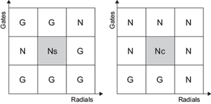
Fig. 1 Isolated noise (left) and continuous noise (right). G refers to good points (non-noisy point, including missing points), N to a noisy points, Ns to isolated noise, and Nc to continuous noise.
In order to solve the problem of continuous noise in dealiasing, an anti-noise velocity dealiasing algorithm (AND) was proposed (section 2). In section 3, five cases were used to illustrate the ability of the AND to repress continuous noise, and its ability to process ambiguity in complex velocity fields. Section 4 provides the summary and conclusions.
2. Algorithm descriptions
The AND is an automatic 3D velocity dealiasing algorithm, which consists of a separation-restoration noise suppression scheme (steps1 and 3 in Fig. 2) and a curve dealiasing method (step 2 in Fig. 2).
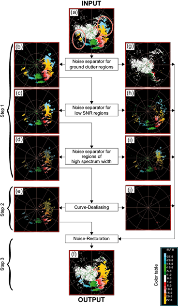
Fig. 2 Schematic diagram illustrating the AND algorithm. (a) raw velocity (red ellipses represent aliased areas), (b) velocity after noise removal in the ground clutter region, (c) velocity after noise removal in the low SNR region, (d) velocity after noise removal in the high-spectrum width region, (e) dealiased velocity from (d), (f) final dealiased velocity, (g) noise in the ground clutter region, (h) noise in the low SNR region, (i) noise in thr high spectrum width region, and (j) velocity without reference velocity or failing in error check.
The separation-restoration noise suppression scheme is one key technique of AND. Traditional noise-filtering algorithms are faced with a contradiction when removing continuous noise. Due to the inability to correctly separate noisy data from non-noisy data, noise suppression methods will mistakenly remove non-noisy data. Usually a more powerful method will lose a larger amount of data. For instance, in the ground clutter region, the noise suppression method will result in loss of data near the zero isodops. Consequently, a contradiction appears: if a small amount of noisy data can be removed, residual noise will still interfere with dealiasing methods; if a large amount of noisy data can be removed, more non-noisy data will be lost. Unlike traditional methods, the separation-restoration noise suppression scheme only separates (step 1 in Fig. 2) and restores (step 3 in Fig. 2) possible noise data, rather than removing them. The only objective of this scheme is to reduce the effects of continuous noise on curve dealiasing (step 2 in Fig. 2); or, in other words, to minimize the occurrence probability of dealiasing errors. The advantage of separation-restoration is that it uses a strict threshold to separate possible noise without losing the good data. Thereby, the contradiction faced by traditional methods is avoided. Specifically, strict thresholds are utilized to separate as many noisy data as possible from raw velocity. Then, after curve dealiasing, all separated possible noise data (including the wrongly removed non-noisy data) are restored to the original positions and dealiased by unambiguous data from step 2 (curve dealiasing).
The flow of the AND algorithm is presented in Figure 2 and the details are described in sections 2.1-2.3. The raw velocities in Figure 2a were used as input for the AND. Two red ellipses contain a blue ambiguous area and a yellow ambiguous area inside. In step1, three noise separators with strict thresholds were used to separate noisy points. First, panel (a) in Figure 2 was separated by noise separators in the ground clutter region into panels b and g. Figure 2b shows the velocities after noise removal, and Figure 2g shows the noise in the ground clutter region. Then Figure 2b was separated by noise separators in the low SNR region into panels (c) and (h). Figure 2c shows the velocities after noise removal, and Figure 2h shows the noise in the low SNR region. Finally, Figure 2c was separated by the noise separator in the high spectrum width region into panels (d) and (i). Figure 2d shows the velocities after noise removal, and Figure 2i shows the noise in the high spectrum width region. In step 2, Figure 2d was dealiased into Figure 2e. Figure 2j shows the velocity without the reference velocity or failing in error check. In step 3, data in Figure 2g, h, i and j were restored into Figure 2e, then each point was dealiased by Figure 2e. Figure 2f shows final velocities after dealiasing. Sections 2.1-2.3 present the details of all steps and thresholds of the AND algorithm.
2. 1 Step 1: noise separation
The causes of noise include ground clutter, low SNR, high spectrum width of target, birds or insects, electromagnetic interference, range folding, super refraction, and measurement errors. Some noise is not essentially noise but a real measurement, such as in the ground clutter region, but it is commonly considered as noise because its radial velocity is largely different from cloud or rain droplets. Noise is divided by three separators, which are applied in the ground clutter, low SNR, and high-spectrum width regions, respectively.
2.1.1 Noise separator for ground clutter regions
A ground clutter region is circumfused with noise, especially continuous noise. Three conditions are defined: (1) The height of echo is below the threshold TGC Hgt (all the thresholds are listed in Table I); (2) reflectivity is above the threshold TGC Z ; (3) absolute velocity is below the TGC Vel threshold. All velocity points that satisfy these three conditions are separated and replaced by a missing value.
Table I Parameters of the AND.
| Threshold | Value | |
| In step 1 | TGCHgt (km) | 1.5 |
| TGCZ (dBZ) | -10.0 | |
| TGCVel (m s-1) | 5.0 | |
| TSNR (dB) | 5.0 | |
| Tsw (m s-1) | 8.0 | |
| In step 2 | TStartAz (deg) | 330.0 |
| TVADPTs | 25 | |
| TMVADPTs | 60 | |
| TβminLen (km) | 20.0 | |
| TβmaxLen (km) | 100.0 | |
| TβdLen (km) | 10.0 | |
| TβPts | 20 | |
| TγminLen (km) | 2.0 | |
| TγmaxLen (km) | 20.0 | |
| TγdLen (km) | 2.0 | |
| TγPts | 8 | |
| TECdiff (m s-1) | Vmax / 2 |
2.1.2 Noise separator for low SNR regions
Due to its low return power, velocity of the low SNR region is usually unreliable, such as velocity data at the echo border. Noise in the low SNR region can be separated by using the method proposed by Gong et al. (2003). First, the reflectivity is transformed to SNR, then the velocity points with SNR below the threshold T SNR are separated and replaced by the missing value.
2.1.3 Noise separator for regions of high spectrum width
High-spectrum width indicates that the target has a highly variable velocity, such as important variations of the wind field or interference by other signals. After the threshold T sw is defined, velocity points with spectrum width larger than T sw are separated and replaced by the missing value.
2.2. Step 2: Curve dealiasing
The curve dealiasing method is another important technique of AND. The key of dealiasing is how to find a reliable reference velocity (V ref ). After step 1 (see Fig. 2e), though noise is removed, there remain abundant missing values that still would lead to unavailable or unreliable V ref . Therefore, a curve-fitting method was designed.
2.2.1 Basic flow
The AND starts from the highest plan position indicator (PPI) at the largest elevation angle in the volume scan, to the lowest PPI. In this study, the elevation angles corresponding to the highest PPI and the lowest PPI are 19.5º and 0.5º, respectively. For each PPI, dealiasing was performed radial-by-radial, clockwise from the azimuth threshold T StartAz , until all radials were finished. For each radial, dealiasing was performed from the point closest to the radar to the one farthest from it.
In the highest PPI, VAD and MVAD were fitted to calculate V ref (section 2.2.2). In other PPIs, three fitting curves were used to calculate V ref (section 2.2.3), including the meso-β line, meso-γ line and VAD curve. The calculation of V ref for the highest PPI is different from the other PPIs. This is because in the highest PPI, the state is unknown for all data, which is either ambiguous or unambiguous. MVAD is more feasible than fitting lines for the highest PPI, because it is very slightly affected by ambiguous data. In other PPIs, since the data of the upper PPI are unambiguous, fitting lines compared with MVAD could more accurately find V ref . If V ref is valid, the Nyquist number is adjusted by Eq. (2), making V T closest to V ref . If V ref is invalid, the current point is separated (into Fig. 2j) and replaced by the missing value. Then error check (see section 2.2.4) was performed. If the current point does not pass the error check, it is separated (into Fig. 2j).
2.2.2 Calculation of V ref based on VAD and MVAD
The reference velocity V ref for the highest PPI was calculated by the VAD and MVAD curves. First, a range ring with the largest number of data was found near the current dealiasing point (± 1 km), then a VAD curve and an MVAD curve were fitted. If the number of data in this range ring is larger than the threshold TVAD PTs / TMVAD PTs , the VAD/MVAD curve is fitted. If both curves are valid, the curve with the smaller standard deviation is selected to calculate the reference velocity V ref at the current position. If only one curve is valid, this curve is used to calculate the reference velocity V ref . If both curves are invalid, V ref is marked as “invalid”.
2.2.3 Calculation of V ref based on three curves
After the highest PPI was dealiased, the V ref of other PPIs was calculated by a meso-β line (20-200 km), a meso-γ line (2-20 km) and a VAD curve. The meso-β and meso-γ lines were least-squares fitting straight-lines along the radial direction. Since a fitting line with the fixed length does not match well with the radial velocity distribution, two length-varying lines were adopted to more accurately find out the V ref . Moreover, the data along the azimuthal direction were also involved by the VAD fitting curve. When the number of radial data was not enough, the VAD curve could provide a reliable V ref .
The procedure for fitting the meso-β line is illustrated in Fig. 3. The meso-β line has four thresholds: Tβ minLen , Tβ maxLen , Tβ dLen , and Tβ Pts . Tβ maxLen and Tβ minLen are the maximum and minimum lengths of the meso-β line, respectively. Tβ dLen is the length increment of the meso-β line, and Tβ Pts is the minimum number of points needed to fit the meso-β line. First, let the searching radius Rs = Tβ minLen and search the dealiased data in the current and the upper PPIs. As shown in Figure 4, there are five round searches centered at the current dealiasing point and in the radius of Rs. Round 1 searches along the current dealiasing radial in the current dealiasing PPI. Round 2 searches along the previous radial in the current PPI. Rounds 3-5 are similar to round 2, except for the upper PPI. If the number of valid points is smaller than Tβ Pts , then extend the searching radius. Let Rs = Rs + Tβ dLen and search five rounds again. Repeat until the number of valid points exceeds Tβ Pts or Rs > Tβ maxLen . After searching, if the number of valid points is larger thanTβ Pts , the least squares method is applied to fit the meso-β line; otherwise the meso-β line is marked as invalid. The meso-γ line is fitted in the same way as the meso-β line, except for the thresholds. The meso-γ line has four thresholds: Tγ minLen , Tγ maxLen , Tγ dLen and Tγ Pts .
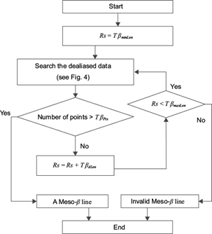
Fig. 3 Flow of fitting meso-β line. Rs is the searching radius. Tβ minLex , Tβ maxLex , Tβ dLex , and Tβ Pts are the four thresholds representing minimum length, maximum length, length increment, and minimum number of points, respectively.
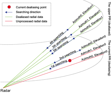
Fig. 4 Illustration of searching dealiased data for fitting meso-β line (meso-γ line). The green lines are dealiased radial data. The red lines are unprocessed radial data. The blue arrowhead denotes the searching direction. Length of the blue line denotes the searching radius. 1st-5th denote round 1-round 5 searching.
The values ref β and ref γ at the current position are interpolated or extrapolated by the two fitted lines. The value refvad at the current position is estimated by using VAD curve. The RMSEs (rms β , rms γ and rms vad ) of the three curves are used as weights, and the reference velocity V ref of the current point is calculated as:
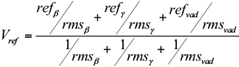 (3)
(3)
If one curve is invalid, the other two curves are used to calculate V ref . If two or three curves are invalid, V ref is marked as invalid.
This method for calculating the reference velocity utilizes azimuthal and radial data, and the weights of three fitting curves, which can dynamically match wind fields of varying scales. For instance, in a velocity field with tornado vortex or large vertical wind shear, the weight of the meso-γ line is larger than those of the other two curves, so the calculation of the reference velocity depends more on the meso-γ line. In a velocity field with ring echoes, radial data have a low coverage rate while azimuth data have high coverage rate, so the calculation of the reference velocity depends more on the VAD curve. When a meso-γ line is invalid or noisy, the meso-β line is bestowed with a large weight, so the calculation of reference velocity depends more on the meso-β line.
2.2.4 Error check
In order to avoid error propagation after dealiasing, the AND immediately checks error after dealiasing one point. This is done by calculating the difference between the dealiased velocity and the V ref . If the absolute difference is above threshold TECdiff, the current point is considered as residual noise and should be separated and filled by a missing value.
2.3 Step 3: Noise restoration
To avoid the influence of continuous noise, the AND separates a large amount of non-noisy data in step1 (see Fig. 2g-i). In order to provide complete information for wind field retrieval and data assimilation, these wrongly separated data should be recovered. After step 2, all data in Fig. 2e are unambiguous, and based on these unambiguous data the AND could easily judge whether a separated point is ambiguous or noise. So, after a separated point is restored to its original position, the V ref at this position is calculated, in the same way as in section 2.2.3, but involving more unambiguous data of upper, current and lower PPIs. Namely, the data in the lower PPI are added to calculate V ref . If V ref is valid, the Nyquist number is adjusted by Eq. (2). If V ref is invalid, the current point is marked as “uncertain”.
3. Case study
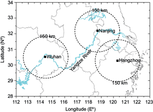
Since 1998, more than 200 operational Doppler weather radars have been installed in China, which constitute the China Next Generation Weather Radar (CINRAD) network. CINRAD-SA is one type of S-band radars located in East China and it is widely used to estimate precipitation, monitor severe weather events and improve numerical weather prediction (data assimilation). CINRAD-SA operates a volume scan at nine elevation angles from 0.5º to 19.5º. The maximum range of the radial velocity field is 150 km (Chu et al., 2014). In this study, three CINRAD-SA radars were selected to evaluate the proposed AND algorithm, including the Wuhan (30.52º N, 114.38º E), Nanjing (32.19º N, 118.70º E), and Hangzhou (30.27º N, 120.34º E) radars (Fig. 5).
The discontinuous stratus velocity field with little or no precipitation is difficult to dealias due to continuous noise and missing data. Thus, three challenging stratus cases were selected to evaluate the anti-noise ability of the AND in this section. Since typhoon and tornado are highly concerned weather events, a typhoon and a tornado case were also selected to illustrate the ability of AND to process velocity fields at different scales. The parameters of AND in these cases were listed in Table I. The current operational dealiasing algorithm of CINRAD is the VDA (velocity dealiasing algorithm) proposed by Eilts and Smith (1990). To validate the improvement of the new method, AND and VDA were compared in each case.
3.1 Dealiasing points near continuous noise
When data is close to the ground clutter region, dealiasing algorithms may produce errors because unambiguous data become ambiguous, or ambiguous data cannot be corrected (Bergen and Albers 1988). In the radial velocity at a 6.0º elevation angle from the Wuhan radar at 17:30 UTC on January 29, 2014, V max is 27.12 m s-1. There is a continuous noise area (white color area circled in a blue ellipse) caused by ground clutter (Fig. 6). Because of the large elevation angle, such noise may come from the side lobe or tail lobe of the antenna. Though weather radars use large-size and high-gain antennas to suppress the side lobe (including tail lobe) power, the side lobe cannot be completely ignored. The most typical phenomenon is the side lobe false echo (DeMott and Rutledge, 1998) when radars observe a strong thunderstorm. Another phenomenon is that in the velocity field, the side lobe will produce large areas of ground echoes with zero velocity. When the elevation angle is raised, the main beam of the radar will not able to contact ground targets, but the side lobe or tail lobe does, which explains the white area within the blue ellipse (Fig. 6). Since velocity of ground targets is largely different from the cloud/rain velocity, here we considered it as noise. Fig. 6a shows two small areas of ambiguous data indicated by red arrows. Under the interference of continuous noise, this case is hard to be dealiased. Fig. 6b is the radial velocity field after dealiasing by operational VDA method. The comparison of panels (a) and (b) in Figure 6 shows that VDA has an obvious error indicated by a red arrow in Figure 6b. However, ambiguous data are well corrected by the AND (Fig. 6c) without influencing any unambiguous data. Since AND integrates the separation-restoration noise suppression scheme, the negative impacts of continuous noise on dealiasing are avoided in this case.
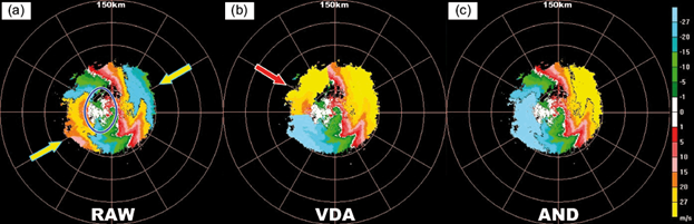
Fig. 6 Radar radial velocity of 6.0º PPI, Wuhan radar, 17:30 UTC on January 29, 2014. (a) Raw velocity, (b) dealiased velocity by the operational VDA, (c) dealiased velocity by the proposed AND. The blue ellipse represents continuous noise caused by clutter from the antenna sidelobe. The yellow arrows show the ambiguous echoes; the red arrows indicate the dealiasing error.
3.2 Dealiasing points in an isolated region
Due to the lack of available reference, isolated echoes are hard to be dealiased. In the radial velocity at a 3.4º elevation angle from the Wuhan radar at 11:49 UTC on January 27, 2014, V max is 27.12 m s-1. This is a stratus case without precipitation. As shown in Figure 7a, five isolated ambiguous echoes (indicated by yellow arrows) exist in the west of the radar, which are overall ambiguous. Namely, the whole echo block has the same Nyquist number. Another ambiguous region is located within 60º-120º (azimuth) and 40-100 km (range). Figure 7b shows a radial velocity field dealiased by traditional VDA. The comparison of panels (a) and (b) in Figure 7 shows that two errors still exist in Figure 7b (red arrows). On the contrary, all ambiguous data are well corrected by AND in Figure 7c, especially the five isolated ambiguous blocks, without influencing any unambiguous data. Since AND uses 3D data at vertical, radial and azimuthal directions, it is very effective in dealiasing isolated echoes in this case.
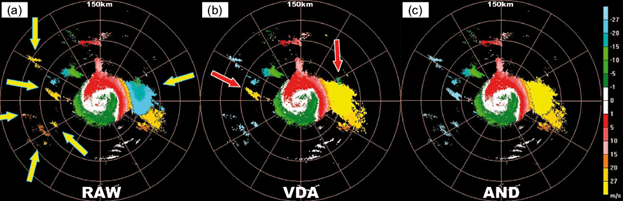
Fig. 7 As in Fig. 6, but for 3.4º PPI from Wuhan radar at 11:49 UTC, January 27, 2014. Yellow arrows show the ambiguous echoes; red arrows indicate the dealiasing error.
3.3 Dealiasing points in the strong wind region
In the radial velocity at a 4.3º elevation angle from Wuhan radar at 04:16 UTC on January 28, 2014, V max is 27.12 m s-1 (see Fig. 8). This is another stratus case without precipitation. Due to the high wind speed (V T ≈ 60m s-1) in the middle and upper air, many ambiguous echoes (yellow arrows) are present, accounting for 1/2 of the echo area. Since V T > 2V max , it is severely ambiguous, so fake zero isodops appeared within 240º-270º (azimuth) and 60-90 km (range) in the ambiguous region. Comparison of panels (a) and (b) in Figure 8 show VDA has corrected the majority of ambiguous echoes, but with an error (red arrow). AND performed better and well corrected all ambiguous points, without changing any unambiguous point. Therefore, AND is also effective for dealiasing in the strong wind region.
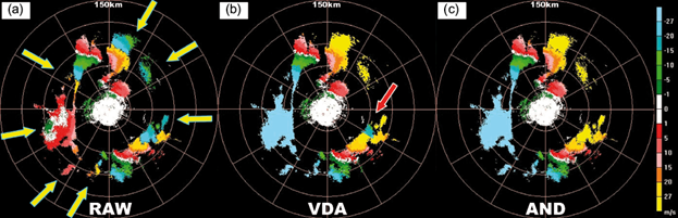
Fig. 8 As in Fig. 6, but for 4.3º PPI from Wuhan radar at 04:16 UTC, January 28, 2014. Yellow arrows show the ambiguous echoes; red arrows indicate the dealiasing error.
3.4 Dealiasing points in the typhoon region
Owing to the large areas and higher reflectivity, dealiasing a typhoon is relatively easy, except for low elevation PPIs. Due to the interference of ground clutters, the typhoon velocity at low elevation angles is usually discontinuous, which easily leads to dealiasing errors. Figure 9 shows the radial velocity of the Chan-hom typhoon an elevation angle of 0.5º observed by the Hanzhou radar. Clearly, Figure 9a reveals three ambiguous velocity zones (yellow arrows). Within the range of 60 km form the radar, the typhoon echoes are mixed with ground clutters (white color). After dealiasing by VDA, the majority of ambiguous data were correctly recovered, but two errors subsist (red arrows in Fig. 9b). On the contrary, AND was not interfered by the low elevation ground clutters and well corrected all ambiguous data. Thus, this case confirms that AND can modestly resist the interference from ground clutters at low elevation angles.
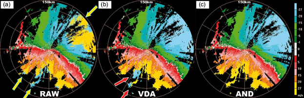
Fig. 9 As in Fig. 6, but for 0.5º PPI from Hanzhou radar at 01:38 UTC, July 11, 2015. Yellow arrows show the ambiguous echoes; red arrows indicate the dealiasing error.
3.5 Dealiasing points in the tornado region
Due to the large horizontal wind shear, a tornado is a challenge for dealiasing algorithms. In the radial velocity at a 1.5º elevation angle in the Nanjing radar at 08:54 UTC on July 03, 2007, V max was 26.37 m s-1 (Fig. 10a). This is a case of an F3 tornado (on the Fujita scale) occurred in the border of Jiangsu and Anhui provinces in east China that killed 14 people and wounded 117. In Fig. 10a, the ambiguous data are located in two areas: the red rectangle and the area between 45º-90º (azimuth) and 120-150 km (range). In Fig. 10c, which is an enlarged image of the red rectangle in Fig. 10a, the tornado is in the red circle, where the blue area corresponds to radial velocity of tornado vortex towards the radar, and it is unambiguous; green area is radial velocity of tornado vortex away from radar, and it is ambiguous. Comparison of panels (a) and (b) in Figure 10 shows that, after dealiasing by AND, all ambiguous velocities are well corrected without changing any unambiguous data. Comparison of panels (c) and (d) in Figure 10 shows that, after dealiasing by AND, the tornado vortex is evident. In the red circle, the green ambiguous data are well corrected, while the blue unambiguous data are unchanged. The results of VDA and AND in this case are similar, thus VDA velocity is not shown in Figure 10. Since AND utilizes three fitting curves to obtain the reference velocity, it can dynamically adapt to varying scales of wind fields, so in this case it is appropriate for dealiasing in the tornado region.

4. Summary and conclusions
Velocity dealiasing of Doppler weather radars is an important quality control method for data assimilation or wind field retrieval. Noise, especially continuous, is an important factor that affects the velocity dealiasing of Doppler weather radars. A challenge in the design of dealiasing algorithms is how to effectively suppress continuous noise. In order to solve the velocity ambiguity in CINRAD-SA operational radars, a novel anti-noise automatic dealiasing algorithm was proposed. The AND utilizes a separation-restoration noise suppression scheme to reduce the interference of noise (especially continuous) without losing any good point. This algorithm utilizes three fitted curves as references to correct ambiguous points. It can further suppress residual noise and dynamically match wind fields at varying scales. After dealiasing by AND, a velocity field preserved the original spatial distribution and positions were consistent with the original data without changing any point (except dealiasing). In order to illustrate the AND’s ability to process complex velocity fields, three stratus cases, one typhoon and one tornado case of CINRAD-SA were analyzed. The results showed that: (1) the negative impacts of continuous noise (including clutter) on dealiasing were avoided due to the separation-restoration noise suppression scheme; (2) since AND uses 3D data at the vertical, tangential and azimuth directions, it is very effective for dealiasing isolated echoes or strong wind echoes; (3) AND is able to dynamically adapt to varying scales of wind fields based on three fitting curves, so it is appropriate for dealiasing in small-scale tornado regions, and (4) as shown in Figures 6-9, the performance of AND is significantly better than the operational VDA.
However, since a large number of curves should be fitted, AND consumes more computing time than traditional algorithms. Furthermore, the patterns of ambiguous velocity fields are very complicated depending on radar parameters, wind field structures and precipitation distributions. According to the statistics of CINRAD-SA data, about 15% of the volume files are ambiguous, and about 75% ambiguity occurs in stratus and weak convections. Ambiguity mainly occurs from December through April (Chu et al., 2014). Only five cases were analyzed in this paper, so more works need to be done, including verification based on a large number data, algorithm optimization, gate-to-gate comparison statistics, etc.

