


 nueva página del texto (beta)
 Inglés (pdf)
 Artículo en XML
 Referencias del artículo
 Enviar artículo por email
 Citado por SciELO
  Similares en
SciELO
Similares en
SciELO 
 Permalink
1. Introduction
Because of its influence on human life, fog has been the focus of many scientific studies. Despite its negative impact on air, road and marine traffic and the associated economic loss, fog is a sustainable hydrological resource for replenishing aquifers, reforestation and for human needs ( Schemenauer and Cereceda, 1991; Gultepe et al., 2007; Möller, 2008; Klemm et al., 2012; Domen et al., 2014).
Many studies and field experiments have demonstrated that the coast of South America exhibits geographical and topographical characteristics that make it suitable for the presence of fog most of the year. The Humboldt Current and the Southeast Pacific anticyclone favor the presence of well-formed stratocumulus clouds that are transported inland by the trade winds and land-sea circulation. When these clouds intercept the coastal topography, advection fog can be observed (Garreaud et al., 2008). Furthermore, when air rich in water vapor is forced by the wind to rise to the prominent relief of the Coast Range it cools, promoting the formation of orographic fogs. Because of these characteristics, patches of diverse fog-dependent plant communities can be observed along the Coast Range in the norcth of Chile. One example is the Fray Jorge Biosphere Reserve located in the Pacific Coast of Chile (30º S) where endemic evergreen tree species grow vigorously (Squeo et al., 2016).
Chile is pioneer in using fog to obtain fresh water for human needs. In 1992, a system of 91 large fog collectors (LFC) were installed in El Tofo, a hill located at 700 masl in the Coast Range of the semi-arid Coquimbo Region. The water harvested from fog was used to provide fresh water to Chungungo, a fishing village with 300 inhabitants, being its only water source during more than eight years (Klemm et al., 2012).
This experience has been replicated in different parts of the world where water is scarce and fog events happen often enough to make the collection of fog water (FW) convenient (Cereceda and Schemenauer, 1991; Schemenauer et al., 1988, 2004; Olivier and Rautenbach, 2002, 2007; Cereceda et al., 2003; Olivier, 2004; Marzol and Sánchez, 2008). Currently, in Morocco and Guatemala there are communities in which the only water source is from fog collected by LFC. The location of sites where fog has been or is currently used as a fresh water source can be found in Klemm et al. (2012).
Technologies to collect FW are simple. The working principle is to expose a mesh to a foggy environment. Water droplets carried by the wind are pushed through the mesh. After successive impacts, the droplets grow by coalescence until they are large enough to fall by gravity and the water can be collected (Rivera, 2011).
The quantity of FW that can be collected in a site is usually measured by a standard fog collector (SFC), a square Raschel mesh with an area of 1 m2 installed two meters above ground level (magl) (Schemenauer and Cereceda, 1994). The collected water can be stored in a container and measured after a period of time, or registered with a pluviometer and a data-logger. SFCs allow the comparison of the potential FW collection in different sites around the world.
Besides the presence of fog, FW collection depends on meteorological variables such as wind speed, wind direction, relative humidity (RH) and/or dew point depression (DPD) (Schemenauer et al., 1988; Schemenauer and Cereceda, 1991, 1993; Cáceres et al., 2007; Hiatt et al., 2012). Other factors that influence FW collection are the orientation of the mesh and its collection efficiency.
The main goal of this paper is to characterize the water collected by an SFC, and to analyze its relationship with local meteorological variables. We analyzed the monthly and seasonal behavior of the FW collection and meteorological variables in a one-year period. The analyzed variables were wind speed, wind direction, temperature, RH and DPD. We further defined a fog index (FI) based in the FW collection, which was compared with the studied meteorological variables.
The research was based on records obtained from an experimental arrangement located in a coastal site of the semi-arid Norte Chico of Chile, consisting on a meteorological station and an SFC.
2. Study site and experimental design
The study site is located on a hill of the Coast Range called El Sarco (29.51º S, 71.27º W, 700 masl), 7 km from the coast and 43 km north of La Serena, the main city of the Coquimbo Region (Fig. 1). The area is characterized by a strong topography gradient with altitudes that vary from sea level to nearly 1000 m in about 10 km horizontal distance. In a macro scale, in the area the Coast Range is narrow, oriented to the NS, and immediately toward the east there is a tectonic basin surrounded by mountains of about 1000 m altitude. Because of these topographic characteristics, the atmospheric variables experience important variations in small distances (Montecinos et al., 2016).
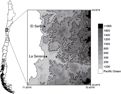
Fig. 1 Study site and its location in Chile. Gray tones indicate the altitude in m, according to the scale shown on the right side. Contour lines are every 400 m.
The climatic characteristics of the area are influenced by the cold Humboldt Current, which moves northwards along the Chilean coast, and the Southeast Pacific high pressure area. At the coast, strong southerly terrain parallel winds are observed (Rahn et al., 2011) and, because of the sea-land circulation, they move eastwards during the day (Montecinos et al., 2016). The annual precipitation near the coast is around 100 mm concentrated in the austral winter months (May to August), and presents strong interannual variations influenced by El Niño-Southern Oscillation (ENSO) (Kalthoff et al., 2002; Falvey and Garreaud, 2007).
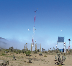
The experimental station is located on a saddle point facing west, between two mountains of around 1000 m altitude. The experimental design is shown in Figure 2. It consisted of a Campbell meteorological station equipped as follows:
Two wind monitors (Young 05106) located at 2.5 and 10 magl, specially designed to work in wet environments, with an accuracy in wind speed and direction of ± 0.3 m s-1 and ± 3º, respectively, and a threshold of 1 m s-1 for the vane.
Two sensors of temperature and RH (model HMP155A) located at 2.5 and 10 magl. The magnitude of errors in temperature depends on the temperature itself: in the range of 0-30º C, the accuracy is smaller than 0.2 ºC. The accuracy of the RH for temperatures ranging between 10 and 25 ºC is ±1% and ±1.7% for relative humidities smaller and larger than 90%, respectively.
A rain gauge (model TE525MM-L25) located at 2.5 magl, equipped with a tipping bucket, with a resolution of 0.1 mm/tip for rainfall (volume per tip: 4.73 ml). The accuracy is ±1, ±3 and ±5% for flows less than 10 mm h-1, 10 to 20 mm h-1, and 20 to 30 mm h-1, respectively.
Near the meteorological station, an SFC oriented in the SW direction (230º) was installed. The water collected by the SFC was measured by a second rain gauge. We highlight that the instrument measures all water that is captured by the mesh or fall into the gutter, therefore it measures both fog and rain water flow. Using the rain gauge of the meteorological station it is possible to know if rain precipitation occurred. Nevertheless, when both fog and rain occurred simultaneously, it was not possible to distinguish the relation between the two water sources using only the two rain gauges.
Both meteorological data and FW collected by the SFC were recorded every 3 s and stored every 10 min.
The results presented in this article are based on data collected in a one-year period, from July 1, 2014 to June 30, 2015. For the purposes of this article, only meteorological variables registered at 2.5 magl were considered.
3. Results and discussion
3.1 Fog water collection
The FW collection presented diurnal and seasonal variations. The maximum FW collected in a 1-h interval was 4.2 L m-2 h-1 and occurred on July 22, 2014 at 0900 LST during a rain precipitation event. Discarding rain precipitations, the highest harvest was 2.6 L m-2 h-1 and happened on September 21, 2014 at 1700 LST. The total FW collection was 1055 L m-2 yr-1, with a mean value of 2.9 L m-2 day-1.
The mean diurnal cycle of the collected FW for each season is displayed in Figure 3. For calculation purposes, the seasons were defined as follows: autumn: March, April, May; winter: June, July, August; spring: September, October, November; and summer: December, January and February. The graphs in the figure show that, on average, in autumn, spring and summer the diurnal cycle presented two maxima, at the early morning and at the evening, with the time when the maxima occurred depending on the season. In winter, the FW collection was smaller than in the other seasons, the variations during the day were smoother and the maximum collection was achieved at the early morning. The four graphs show that the standard deviations (STDs) of FW collection are larger than the hourly mean values. Notwithstanding the high STD, we also observed two maxima in autumn, spring and summer, but in winter there was not a clear variation in the collected water. When the STD was normalized with respect to the mean value, we found that: i) the dispersions are larger during the day than at night, and ii) the deviations in winter are larger than in summer time (not shown). This fact is related to the variations of the liquid water flux (LWF), which depends on the wind speed and fog liquid water content (LWC), which was not measured in this study. We note that the accuracy of the instrument is much smaller than the STD, thus it can be neglected for the data analysis.
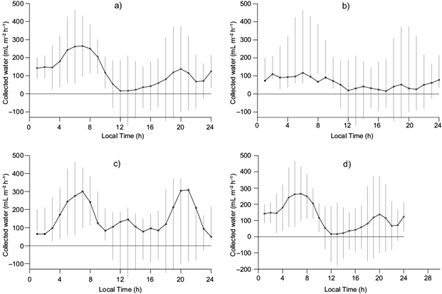
Fig. 3 Seasonal mean diurnal cycle of the FW collected by the SFC: (a) autumn, (b) winter, (c) spring, and (d) summer. Vertical lines represent the standard deviation of the mean (STD).
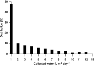
In Figure 4, the distribution of the daily volume of FW collection is displayed. We found that 47.3% of the days of the year the quantity of collected water was less than 1 L. The distribution showed a sharp decline between the first value and the next one, and from there on a slow decrease was appreciated. The maximum collection was 12 L m-2 day-1.
Garreaud et al. (2008) defined a qualitative fog index (QFI) as the number of foggy days per month, and a foggy-day was defined as a day when three visual observations performed by rangers in the Fray Jorge Biosphere Reserve detected the presence of fog. These authors showed that there exists a direct relation between the QFI and the FW collected by passive fog collectors.
In this article, we define an FI based on quantitative observations as the percentage of foggy-days per month, and a foggy-day as a day in which the water collected by the SFC is more than 1 L m-2. After Figure 4, 53.7% of the days of the year were foggy-days. In Figure 5, the FI and the total water collected by the SFC per month are displayed. For reference, the accumulated rain precipitation per month, as registered by the rain gauge of the meteorological station, is also presented. In general terms, we found similar FI values over the year - ranging between 23.3 and 77.4% -, with the exception of winter months, when they were smaller. The monthly FW collection fluctuated between 21.3 and 154.5 L m-2. Both FI and monthly FW collection reached the minimum and maximum values in June and January, respectively.

3.2 Air temperature and relative humidity
The 10-min intervals averaged temperature ranged between 3.7 and 29.6 ºC, and the RH fluctuated between 5% and saturation values, with the minimum values achieved in winter (not shown).
In Figure 6, the monthly mean temperature and RH are presented. As it can be observed, temperature experienced two peaks (in March and June) with values of 14.7 and 13.8 ºC, respectively. The minimum mean monthly temperature was 10.4 ºC and, considering the dispersion given by the STD, it was reached from July through September. The minimum and maximum values of the monthly mean RH were 55.8 and 94.1%, achieved in June and January, respectively.
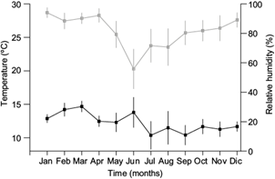
The presence of fog is related with high values of RH. If we compare Figures 5 and 6, it can be observed that the behavior of the monthly RH follows the same trend as the FI. Discarding winter, and in a lesser extent, the temperature follows an opposite trend with respect to the FI. During winter months, STDs are too large to find a relationship between temperature and FI.
Further, we found that the monthly daily temperature amplitude was larger in the austral winter than in the summer months (not shown). The same behavior can be observed in Figure 6 for the STDs of both monthly temperature and RH. The smaller fluctuations of both temperature and RH observed in the summer months could also be related with the higher frequency of fog episodes observed in summer than in winter, as we will discuss in section 3.4.
Figure 7 displays the mean diurnal cycle of temperature and RH in winter and summer. As it can be observed, and similarly to the monthly mean values, the STDs of both variables are larger in winter than in summer. In both summer and winter the temperature is larger during the day than in the night hours but, because of the large STD observed especially in summer, it is not possible to compare the temperature values between winter and summer time. In the case of the RH, in summer the averaged values are higher than 84%, whereas in winter they ranged between 62 and 69%. The high values of RH in summer can be related to the higher frequency of fog episodes observed in the same period.
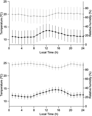
Fig. 7 Mean diurnal cycle of temperature (black) and RH (grey) in winter (above) and summer (below). The vertical lines represent the STD.
The low values of RH in the austral winter time (observed in Figs. 6 and 7) suggest a decrease of the specific humidity in winter, probably due to a lower evaporation of water from the ocean.
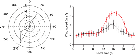
3.3 Wind speed and wind direction
The wind characteristics were compatible with the land-sea circulation. During the day, the wind blew from sea to land (SW) and at night in the opposite direction (NE), as it can be seen in the wind direction distribution displayed in the left panel of Figure 8. The wind speed in 10-min averages ranged between calm and 13.1 m s-1 (not shown), stronger during the daytime than at night. This behavior can be observed in the right panel of Figure 8, which shows the mean diurnal cycle of the wind speed in the austral winter and summer time, with the corresponding STDs. As observed in the figure, the STDs of the hourly wind speed were larger in summer than in winter, and larger than the accuracy of the instrument.
3.4. Fog water collection and meteorological variables
The collection of FW occurs when air rich in water droplets crosses the mesh. The LWF across the mesh depends on the wind velocity and the LWC in fog (Park et al., 2013). For this reason, despite that the arrival of fog and the collection of FW are not simultaneous events, some relation between the collection and meteorological variables is expected.
Figure 9 displays the diurnal cycle of wind speed, FW collected by the SFC, temperature and RH on September 21, 2014, the day of maximum-recorded FW collection without rain precipitation.
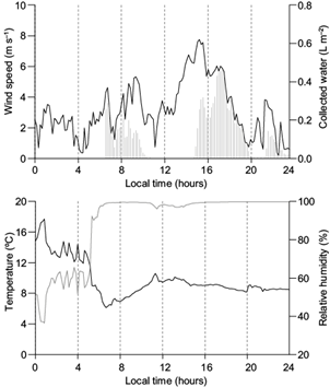
Fig. 9 Diurnal cycle of meteorological variables on September 21, 2014. Above: wind speed (line) and collected FW (vertical lines). Below: temperature (black) and RH (grey). The data correspond to 10-min intervals.
The down panel on Figure 9 shows that at about 0600 LST the RH reached values above 95%, which could be related with the beginning of a fog event. Thereafter, RH experiences small variations, so it could be supposed that fog occurred all day until midnight. During this period with saturated conditions, relatively small variations of temperature were observed.
At the up panel of the figure, it can be observed that the FW collection started at 0700 LST, also one hour after saturated conditions were achieved, which suggests that there exists a lag between the arrival of fog and the start of the collection, and agrees with observations performed by the authors using a fog monitor. After that, the collection roughly followed the behavior of wind speed. The collection stopped when the wind speed achieved values of around 1 m s-1, coincident with a change of the wind direction from the NE (not shown). It started again at about 1500 LST after an increase in wind speed. At 1600 LST, both wind speed and water collection decreased, and the collection ceased when the wind speed was around 1 m s-1. At the evening a third episode of FW collection can be observed.
The behavior observed in Figure 9 and described above, can be understood if we consider the physical processes involved in the FW collection. This happens when the water droplets in the air flux impact the collector and the droplets trapped by the mesh grow by successive impacts until they are large enough to fall in the gutter, where they are conducted to the container, passing by the detection system (rain gauge). Hence, the decrease in the FW collection when the wind speed decreases, can be due to a decrease in the LWF that reaches the mesh. Further, the time needed in all the involved processes, from the beginning of the fog events and the start of the collection, depends on the characteristics of the mesh and the fog and environmental conditions. The description of the detailed processes falls beyond the scope of the present investigation.
Another factor that influences FW collection is the collection efficiency of the system, defined as the ratio of collected water to LWF over a given time. Depending on the prevailing meteorological variables and fog microphysical characteristics, different processes occur - each with its own efficiency (Rivera, 2011; Park et al., 2013) - during the time it takes for the LWF to reach the SFC before finally being detected by the rain gauge. For example, Schemenauer and Joe (1989) showed that the collection efficiency depends on the mean volume diameter of the fog droplets and the wind speed.
Figure 10 displays the relationship between collected water and wind speed (left panel) and wind direction (right panel). The vertical dashed lines in the right panel represent the orientation of the SFC. Because of the lag between the arrival of fog and the beginning of the collection, collected water in one-hour intervals and the mean values of wind speed and wind direction in the same period are represented.

Fig. 10 FW collection and wind speed (left) and wind direction (right) as one-hour averages over the full year of study. The vertical dashed line in the right panel indicates the orientation of the mesh.
In the left panel of the figure it can be seen that, for each value of wind speed, the collected FW varied from zero to a maximum value, which increased with wind speed. This result can be explained because the LWF is proportional to the wind speed, the projection of the air flux over the normal to the mesh, and the LWC. Further, the number of water droplets in the air flux that achieve the final collection system depends on the mesh collection efficiency. Roughly, we can also conclude that, for a fixed wind speed, the FW collection increases from zero (when no fog is present) with the increasing fog LWC.
Regarding to the relationship between FW collection and wind direction displayed in the right panel of Figure 10, we found that collection occurs both when the wind is coming from the SW and from the NE. The figure shows that the maximum collection occurred for a wind direction of 225º, suggesting it may increase if the SFC were rotated about 5º counterclockwise with respect to the current orientation (230º). Nevertheless, because of the error of the vane of ±3º, the evaluation of the best mesh orientation needs further research.
In Figure 11, the relationship between FW collection and DPD as one hour averages is presented. The figure shows that the FW collection occurs mostly for low values of DPD, which agrees with the results found by Hiatt et al. (2012). Nevertheless, it can occur also for values of DPD of up to 8 ºC. This result could be explained because, despite that the presence of fog occurs under saturation conditions (which means values of DPD near zero), collection and fog events are in general not simultaneous. In fact, after observations performed by the authors using a fog monitor, water drainage in the SFC may continue for nearly one hour after the fog event has stopped.
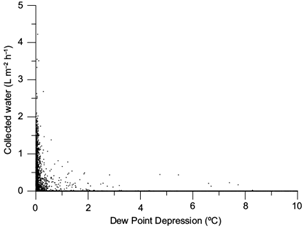
Fig. 11 Relationship between FW collection and DPD as one-hour averages over the full year of study.
Figure 12 displays the relation between the FI and the daily temperature amplitude per month (dT). As observed, FI decreases by increasing dT. The linear regression that describes the relation between FI and dT is:

FI (%) =− 7.3 × dt + 103.1, (1)
with dT in ºC. The root mean square error for (1) is 9%. This can be explained because of two factors: (1) the heat capacity of moist air is larger than that of dry air and, therefore, the former cools and heats more slowly than the latter; and (2) fog, as all clouds, both prevents cooling by radiation during the night and attenuates the incident solar radiation during the day due to reflection (Lamb and Verlinde, 2011).
The decrease of temperature variation when FW collection occurs can also be observed in particular days, as shown in Figure 9. Similarly, the smaller STD of temperature observed in summer months than in winter can be as well related to the higher frequency of fog episodes recorded in the same periods.
4. Conclusions
In this paper, the FW collected by an SFC and its relationship with local meteorological characteristics were analyzed. The results were based on records obtained in a one-year period.
The principal findings were:
The seasonal diurnal cycle of the FW collection presented variations during the year. In the austral autumn, spring and summer it peaks twice: in the early morning and in the evening. In winter, the collection is less than in the other seasons, and experiences small variations during the day.
We found that 53.7% of the days of the year were foggy-days. The FI is larger in the austral autumn and winter than in the spring and summer months. It ranged between 23.3 and 77.4%, achieved in June and January, respectively. The FI and the monthly FW collection follow the same trend, with minimum and maximum achieved in the same month, which agrees with results found by Garreaud et al. (2008).
The monthly mean RH ranged between 55.8% and 94.1%, larger in summer than in winter, which is related to the higher frequency of fog episodes observed in summer than in the winter months.
For each value of wind speed, FW collection varied from zero up to a maximum value, which increased with wind speed. This behavior can be explained because the LWF increases with wind speed and LWC in the flow. Roughly, for a fixed wind speed, higher collection corresponds to higher values of LWC.
FW collection occurred both for wind coming from the SW and the NE.
Mostly, FW collection happened for values of DPD near zero. However, collection can happen for values of DPD of up to 8 ºC, which can be due to the fact that FW collection and the presence of fog are not always simultaneous events, since FW collection was observed to occur also after the fog event had stopped.
The FI increased with decreasing monthly daily temperature amplitude, which is due to the fact that wet air heats and cools more slowly than dry air, and fog prevents the nocturnal cooling by radiation and diurnal heating by reflecting the incoming sun radiation.
Finally, we stress the fact that both meteorological characteristics and FW collected in the study site are based in a one-year period, so that interannual variations cannot be considered.

