


 text new page (beta)
 English (pdf)
 Article in xml format
 Article references
 Send this article by e-mail
 Cited by SciELO
  Similars in
SciELO
Similars in
SciELO 
 Permalink
1. Introduction
The planetary boundary layer (PBL) is the lowest layer of the troposphere that is directly influenced by its contact with the earth’s surface. The height of the PBL is a crucial parameter for air quality analysis, pollutants dispersion and quantification of pollutant emissions and sources (Coen et. al., 2014). The role of convective boundary layer is more pronounced over tropical regions (like India) in comparison to other parts of the world. The meteorological processes within the PBL influence the transport and chemistry of air pollutants (Reddy et al., 2012). Significant work has been done around the world on the influence of boundary layer phenomena and meteorology on the characteristics of air pollution and the status of air quality (Kolev et al., 2011; Quan et al., 2013).
Surface emissions of major air pollutants have been changing substantially over the tropical region in the past few decades. The global epidemiological study on the effect of air pollution revealed that particulate matter and gaseous pollutants could cause severe health effects (particularly in urban areas) like respiratory and cardiovascular diseases, resulting in cardiopulmonary mortality (Dockery et al., 1993; Koken et al., 2003). Concern about air pollution in urban areas is receiving increasing importance world-wide, especially pollution by gaseous and particulate trace metals (Azad and Kitada, 1998; Salam et al., 2003; Begum et al., 2004).
Systematic air quality monitoring programs have also been perfomed in different developing countries like Bangladesh and Pakistan (Ali and Athar, 2008; Salam et al., 2008). In India, air pollution has increased rapidly with population growth, increasing number of motor vehicles, use of fuels with poor environmental performance, badly maintained transportation systems, poor land use pattern, and above all, ineffective environmental regulations (Ghose et al., 2004; Gupta et al., 2008). Stationary and mobile sources emit a wide variety of pollutants, principally carbon monoxide (CO), nitrogen oxides (NOx), sulphur oxides (SOx), volatile organic compounds (VOCs) and particulate matter, which have an increasing impact on urban air quality. In addition, photochemical reactions resulting from the action of sunlight on nitrogen dioxide (NO2) and VOCs emitted by vehicles lead to the formation of ozone, a secondary long-range pollutant, which impacts rural areas often far from the original emission site. Systematic analysis has shown that boundary layer characteristics and meteorological parameters strongly influence the variation of surface ozone (Reddy et al., 2012; Ghosh et al., 2013, 2015). Long-range horizontal transport also plays a crucial role in the variation of ground level ozone concentration (Ghosh and Sarkar, 2015). Many researchers have focused on the monitoring and analysis of air pollutants and air quality in different parts of India like Kolkata, Delhi, Lucknow, Haryana, Chennai, Mumbai, Dhanbad-Jharia, Raniganj-Asansol, Durgapur and Burdwan (Lal and Patil, 2001; Jain and Saxena, 2002; Goyal and Sidhartha, 2003; Reddy and Ruj, 2003; Verma et al., 2003; Kaushik et al., 2006; Pulikesi et al., 2006; Gupta et al., 2008; Chattopadhyay et al., 2010; Dey et al., 2014, 2017).
Durgapur is one of the most polluted cities of the country with a cluster of industries. It is located in the eastern part of the country. So far no systematic air quality-monitoring program with a Geographic Information System (GIS) approach has been reported from this region. Therefore, systematic as well as scientific investigation of the ambient air quality status of different areas (with high vehicular density, residential and industrial) is essential to formulate a proper mitigation strategy for pollution.
The present study focuses on the variations in the concentration of particulate matter (PM10) and various gaseous pollutants (SO2, NO2, CO, NH3 and O3) over an urban region of eastern India and attempts to find the influences of meteorology and planetary boundary layer characteristics on dispersion and dilution of pollutants near ground level. It also aims to explore the probable sources of air pollutants and the air quality status of the three different sites under consideration. Various statistical techniques are used for understanding the relationship between concentration of air pollutants, meteorological variables and PBL characteristics. Computation of the air quality index (AQI) for each of the three chosen sites is done.
2. Materials and method
2.1 Site description
Data were collected at three different sites (Fig. 1) of an urban area in eastern India during April and May, 2014. These sites are located in Durgapur (Burdwan district) of West Bengal. Site I (Faridpur) is situated at 23º 32′ 27.61ʺ N and 87º 17′ 7.28ʺ E. The sampling site is adjacent to National High Way (NH-2) or the Grand Trunk Road. This site represents an area with high vehicular density.

Site II (B Zone) is located at 23º 33′ 53.79ʺ N and 87º 19′17.26ʺ E. This site is situated in a residential area which is far away from national highway and industrial area.
Site III (DVC-DTPS Colony) is situated in an industrial area at 23º 31′ 19.42ʺ N and 87º 15′ 33.59ʺ E. River Damodar flows to its south. The Durgapur Steel Plant (DSP) and the Durgapur Thermal Power Station of the Damodar Valley Corporation (DVC) are close to this site
2.2 Meteorological background
This area undergoes hot and dry summers, lasting from March to the middle of June, with average daily temperatures near 32 ºC, followed by the monsoon season with heavy precipitation and somewhat lower temperatures. Durgapur receives most of its annual rainfall of around 32 mm during this season. The monsoon is followed by a chilled dry winter from November to January. Temperatures are quite moderate, with average daily temperatures near 20 ºC. There is a short autumn at the end of October and a short spring in February, both of which have relatively moderate temperatures of around 25 ºC. This area with undulating topography is covered with red and yellow Ultisol soils, with an average elevation of 65 masl.
2.3 Measurement techniques
Various criteria pollutants and meteorological parameters were monitored at these three different sites from April to May 2014. Sampling was carried out at each site for 10 consecutive days. Monitoring of PM10, SO2, NO2, O3, CO, NH3, and meteorological parameters (temperature, humidity, wind speed and direction) was performed for 24 h. Data were collected on the roof of single-story buildings in all the three sites.
The concentration of PM10 was obtained with the aid of a high volume sampler (Envirotech APM 460BL) from Envirotech. Air was drawn through a size-selective inlet and through a 20.3 × 25.4 cm filter paper (GF/A) at a flow rate which is typically 1132 L/min. The high volume sampler was run in the open air for 24 h and initial and final flow rate values were recorded. The collection interval of PM10, SO2 and NO2 was 24 h. After the required time of sampling, the filter paper was taken out and stored carefully in an envelope within the desiccator for subsequent analysis. Particles with aerodynamic diameters less than a cut-point of the inlet were collected by the filter. The mass of these particles was determined by the difference in filter weights prior to and after sampling. The concentration of suspended particulate matter in the designated size range was calculated by dividing the weight gain of the filter by the volume of air sampled.
SO2, NO2 and NH3 were monitored with the same kind of high volume sampler. Twenty-five millimeters of potassium tetrachloromercurate (TCM) absorbing solution were placed in an impinger and sampled for 24 h. A calibrated flow-measuring device was used to control the airflow from 0.2 to 1.0 L/min. The volume of the sample was then measured and stored in a sample storage bottle. The chemical analyses of samples and blanks were performed in the laboratory (West and Gaeke, 1956) for estimation of ambient SO2 (µg m-3) concentration. The absorbances of the solutions were measured at 560 nm.
Ambient air was continuously drawn into 25 ml of a sodium hydroxide solution for analysis and estimation of NO2 concentration. The flow rate of ambient air was 0.2-1.0 L/min and was controlled by a calibrated flow measuring device. The samples and blanks were chemically analyzed and the concentration of the nitrite ion was determined by colorimetric analysis (Jacobs and Hochcheiser, 1958). The absorbances of the solutions were measured at 540 nm.
The concentration of ambient ammonia was determined by the indophenol blue method in the laboratory. Ambient air was continuously drawn into 25 ml of a dilute solution of sulphuric acid with a flow rate of 1-2 L/min and sampled for one hour. The ammonium sulphate thus formed in the sample was allowed to react with phenol and alkaline sodium hypochlorite to produce indophenol. Sodium nitroprusside acts as catalyst in this reaction. The estimation of NH3 is done by measuring the absorbance of the samples and the blanks at 630 nm (Lodge, 1998). The absorbance of all the samples and blanks for the estimation of SO2, NO2 and NH3 was measured by means of a UV-VIS spectrophotometer (Lambda 35, Perkin Elmer).
The concentration of O3 was continuously monitored with the help of an air quality sensor (Aeroqual series 500). The sampling was carried out for 24 h with a sampling interval of 1 h.
The concentration of CO was measured with a lightweight portable indicator (PPSMPL gaZguardTx). The sampling of CO was performed for 24 h with a sampling interval of 1 h.
Meteorological parameters such as humidity, temperature, and wind speed and direction were also recorded during the sampling time. Humidity and temperature were measured with portable hygrometer (Model-HTC-1), wind speed was measured with a digital anemometer (Lutron-AM-4201) and wind direction was recorded with a wind vane. The portable hygrometer, digital anemometer and wind vane were all placed on the roof of single story buildings (approximately 3.5 m above the ground level).
To ensure the quality of the laboratory analysis of air pollutant samples, pure chemicals of AR grade (Merck, Germany) were used. Low actinic glassware was used during the analytical analysis of the samples. The quality of the titrimetric method was maintained by considering the mean titre value obtained by averaging the three concordant titre values. Different instruments used during sampling (i.e., the Aeroqual high volume sampler and the gaZguardTxlightweight portable indicator) were properly maintained and calibrated in order to fulfill the quality control requirements.
Data of parameters like PBL height, vertical mixing coefficient and cloud cover for the specific days of observation over the sites of interest were collected from the archived data of NOAA’s Air Resources Laboratory (https://ready.arl.noaa.gov). The data of sunrise and sunset over the three sites during the study period were collected from the site of NOAA’s Earth System Research Lab (http://www.esrl.noaa.gov/gmd/grad/solcalc/sunrise.html). Wind rose diagrams were constructed with the monitored data (wind direction and speed) for the study period using the WRPLOT View software (v. 7.0.0).
2.4 Statistical analysis
The primary data set was processed and analyzed with different statistical tools to obtain their descriptive statistics.
2.4.1 Multivariate statistical analysis
Principal components analysis (PCA) is a multivariate statistical procedure designed to classify variables based on their correlations. The goal of PCA and other factor analysis procedures is to consolidate a large number of observed variables into a smaller number of factors (components) that can be more readily interpreted as the underlying processes. The XLSTAT 2012 statistical software was used to perform PCA, specifying the principal components method with varimax rotation (Kaiser, 1958). The rotation of the component axis is performed so that components are clearly defined by high loadings for some variables and low loadings for others, facilitating the interpretation in terms of original variables.
2.5 Air quality index (AQI)
An AQI could be defined as a scheme that transforms the (weighted) values of individual air pollution related parameters into single number. Initially, the air quality rating of each parameter used for monitoring is determined in each site by the formula
 (1)
(1)
where q is the quality rating, V the observed value of the parameter and Vs the value recommended for that parameter.
The geometric mean of ‘n’ number of quality ratings was determined by
 (2)
(2)
where g is geometric mean; a, b, c, d, and x are different values of air quality ratings; n is the number of values of air quality ratings, log is the logarithm function and antilog is its inverse.
The air quality status of different sites is determined on the basis of the AQI categorization proposed by Mudri (1990) (Table I).

2.6 Backward trajectory simulation
An air mass backward trajectory analysis was carried out to identify the sources and pathways of air pollutants. The simulation was done using NOAA’s HYbrid Single-Particle Lagrangian Integrated Trajectory (HYSPLIT) model (Draxler and Hess, 1998) with GDAS meteorological data. The 10-day back trajectories at three altitude levels (100, 500 and 1500 m above the ground level) are simulated for all three sites.
3. Results and discussion
3.1 Variation of the gaseous pollutants and particulate matter concentrations over the three sites
PM10, O3, SO2, NO2, CO, and NH3 are some of the major air pollutants which require monitoring and analysis to understand the air quality status of an area.
3.1.1 Influences of PBL characteristics on pollutant concentrations
Gaseous NH3 has long been known to play a key role in atmospheric chemical processes. NH3 is a major contributor to secondary aerosol formation in the atmosphere. Anthropogenic sources of ambient ammonia include industrial processes, vehicular emissions and volatilization from soils and oceans (Behera et al., 2013). CO and NO2 are the primary air pollutants, which are directly emitted into the air. The major anthropogenic source of CO and NO2 is the burning of fossil fuels (combustion in motor vehicles). The primary sources of SO2 are burning of fossil fuels and petroleum products, as sulfur is present in these products as impurities.
Variations in concentration of air pollutants (NO2, SO2, NH3 and CO and PM10) and average PBL heights over sites I, II, and III during the study period are plotted in Fig. 2a, b, c, respectively.

Fig. 2 Day-to-day variations of different air pollutants and PBL heights during the study period over (a) site I (Faridpur), (b) site II (B zone), and (c) site III (DVC-DTPS Colony).
The concentration of NO2 is found to be high in sites I and III. Forty percent of the obtained values of NO2 in site I exceeded the National Ambient Air Quality Standard (NAAQS) limit and 50% of the monitored values exceeded the NAAQS limit in site III. However, in site II the concentration of NO2 is much lower than the permissible limit. The concentration of NH3 is lower than the NAAQS permissible limit in all three sites. The 24-h average level of NH3 is highest in site I (109.7 µg m-3 and a range of 17.1-231.8 µg m-3) and lowest in site II (with a 24-h average of 13.6 µg m-3 and a range of 4.2-29.2 µg m-3). The maximum SO2 concentration was found at site III (industrial area) with all values exceeding the NAAQS permissible limit. A similar kind of result was also found by Chattopadhyay et al. (2010). In sites I and II, the SO2 level is much lower than the permissible limit. The average hourly concentration of CO in the ambient air was lowest in site II (0.6 µg m-3) and highest in site III (3.8 µg m-3). Only 10% of the monitored data exceeded the NAAQS limits at site III whereas concentration values in sites I and II did not exceed the limits prescribed by NAAQS. High PM10 levels were observed in all three sites. The highest average PM10 level was observed at site III (392.1 µg m-3 with a range of 247.8-499 µg m-3) and all the monitored values exceeded the permissible limits. The lowest PM10 level was found at site II with a mean of 85.7 µg m-3. Only 40% of the monitored values exceeded the NAAQS limits at this site. In site I, 80% of the monitored values exceeded the permissible limits. Although the estimation of ammonia emissions to the atmosphere is characterized by a high degree of uncertainty, the transportation sector is believed to be the largest contributor to urban emissions of this compound. As site I is adjacent to a national highway (NH-2), comparatively higher concentrations of ambient NH3 are found over this site than in the other two sites. Ambient NH3 contributes to increase PM concentrations in the urban atmosphere (Walker et al. 2004; Whitehead et al., 2007). The presence of high NH3 levels at site I also contributes to a high PM10 concentration at this site. High traffic density also enhances the concentration of CO and NO2 over this site.
High concentrations of SO2, NO2, CO and PM10 were recorded at site III (Fig. 2c). The burning of fossil fuels in various industrial processes produce huge amount of sulfur oxides, nitrogen and carbon. Therefore, industrial activities near site III account for the high concentration of SO2, NO2, CO and PM10 in the ambient atmosphere of this site. Local biomass burning and domestic coal burning might be the cause of the occasional presence of very high values of these air pollutants.
Boundary layer characteristics also play a crucial role in the dispersion and dilution of air pollutants near the earth’s surface. It is observed that days with higher average PBL height show lower pollutant concentrations near the ground (Fig. 2a, b, c). Higher average PBL heights and enhanced convective activities facilitate the dilution of pollutants, thereby decreasing their concentration near the earth’s surface, whereas in days with lower PBL height pollutants get trapped near the ground.
3.1.2 Diurnal variation of ground level ozone concentrations over the three sites
The diurnal variation of ground level ozone at sites I (Faridpur), II (B zone), and III (DVC- DTPS residential area) are shown in Figs. 3, 4 and 5, respectively.

Fig. 3 Diurnal variation of ground level ozone concentration at site I (Faridpur) during the study period.

Fig. 4 Diurnal variation of ground level ozone concentration at site II (B zone) during the study period.

Fig. 5 Diurnal variation of ground level ozone concentration at site III (DVC-DTPS residential area) during the study period.
In general, contour diagrams show that ozone concentration begins to increase gradually after sunrise, attains a maximum around noontime and starts decreasing after late afternoon or evening. Sunrise and sunset times during the study period over the three sites are reported in Table II.

The daytime increase in ozone concentrations, which is a pronounced feature of urban polluted areas, is basically due to the photo oxidation of precursor gases such as CO, CH4, and non methane hydrocarbons (NMHCs) in the presence of a sufficient amount of NOx (Lal et al., 2000).
Ozone concentration is highest around noon and in the afternoon (12:00-16:00 LT) in all three sites. Meteorological factors, boundary layer processes and regional/long range transport play vital roles in determining the ozone concentration depending on the topography of the observational sites. After sunrise, the boundary layer height gradually increases from 200-300 m to about 1500-2000 m during noon hours due to convective heating and the stratification of layers (Lal et al., 2000). During noon hours, air rich in ozone in higher altitudes mixes with the air in lower altitudes, which has a lesser amount of ozone (Naja and Lal, 1997). During nighttime, the photochemical production of ozone ceases and vertical transport of this element is inhibited by a nocturnal inversion layer. Loss of ozone by reaction with NO (titration) and dry deposition are the other causes of low ozone concentration during nighttime. Low ozone concentrations during early morning are due to the combined effects of suppressed boundary layer mixing processes and chemical loss by reaction with NO.
3.1.3 Site-specific variation of ground level ozone concentration
Site III (DVC-DTPS residential area) shows the highest hourly averaged ozone concentration followed by sites II and I. Urban quenching (Schneider et al., 1988) appears to play a major role in the high ozone levels measured in site II. This seems to occur because there is so much NO in the atmosphere over sites I and III (from vehicular and industrial emissions, respectively) that ozone reacts immediately with this compound (NO +O3 → NO2 + O2). Table II shows that sunset time ranged from 18:08 to 18:12 LT over site II during the sampling period. The source of nocturnal ozone might be the long range of ozone transport. However, high concentrations of ozone over site II persist even after sunset (Fig. 4).
A ten days air-mass backward trajectory simulation was performed to ascertain the source and transport pathways of gaseous pollutants. The back trajectory analyses depicting the air mass trajectory at three different levels (100, 500 and 1500 m) over the three sites are shown in Fig. 6a, b, c, respectively.

Fig. 6 Back trajectory analyses depicting the air mass trajectory at three different levels (100, 500 and 1500 m) over (a) site I, (b) site II and (c) site III.
Figure 6b shows that during the study period air masses at 100 and 500 m predominantly originated from the Bay of Bengal, entered the continental land mass through Andhra Pradesh and reached site II after travelling through Jharkhand, Chattisgarh and other provinces. These are highly industrialized areas with plenty of iron, steel and chemical industries, power plants, etc., which are known to be major sources of most of the precursors of daytime ozone. The air mass at 1500 m originated from Iran and traveled through arid regions of Pakistan and the desert of Rajasthan, entering site II. During its passage over the continental landmass, it was exposed to local pollution and accumulated precursors of daytime ozone, which resulted in the formation of ozone under favorable meteorological conditions. This might be the reason of enhanced ground level ozone over site II. The wind rose diagram in Figure 7b shows that wind predominantly flowed in the W-SW direction (244º) over site II during the study period, which further confirms the transport of ozone from other regions. Site III is surrounded by a large number of industries (iron, steel, and alloy industries, among other industrial facilities), which are the major sources of daytime ozone precursors. The presence of high concentrations of precursors along with favorable meteorological conditions enhances the photochemical production of daytime ozone. Moreover, the back trajectory simulation depicts that the air mass at 100 and 500 m originated from arid regions in Rajasthan and Afghanistan, respectively, and reached site III after passing over Jammu, Kashmir, Uttar Pradesh, and Bihar. The air mass at 1500 m originated at the Arabian Sea near Somalia, crossed it and passed over Rajasthan, Uttar Pradesh and Bihar, arriving to site III. The high concentrations of ground level ozone at site III may be due to these air masses . The wind rose diagram of site III (Fig. 7c) shows that the dominant wind direction is W-NW (292º). The 10-day back trajectory air mass simulation clearly depicts that air masses at 100 and 500 m have mostly passed over the Bay of Bengal before reaching site I, and they have not circulated over the continental regions of India long-enough to be exposed to local pollution, which results in low ozone concentrations over site I. The wind rose diagram of site I (Fig. 7a) further confirms that wind predominantly flows in the S-SW direction (209º).

3.1.4 Daily variation of ground level ozone and PBL characteristics
The daily variation of ground level ozone concentrations along with daily averages of PBL height and vertical mixing coefficients over sites I, II, and III are shown in Figure 8a, b, c, respectively. Apart from in situ photochemical production of tropospheric ozone, this element can be transported downward from the stratosphere (Reddy et al., 2012). Tropospheric photochemical production of ozone is the dominant source while boundary layer dynamics plays a crucial role in controlling the ground level ozone concentration. The vertical mixing coefficient is the measure of turbulent mixing within the boundary layer and gives an idea of vertical movement of the pollutants. It is actually mixing length times the velocity of wind within the mixing length, which can be defined as the depth, measured upward from the earth’s surface through which pollutants are vigorously mixed (Rao et al., 2003). The vertical mixing coefficient determines the air pollution potential of an area. The PBL starts evolving after sunrise, attains a maximum height during afternoon due to surface heating and again decays after sunset. During afternoon hours, the turbulent mixing in the convective boundary layer enables the vigorous mixing of the chemical species present within the boundary layer depth. This process significantly affects the ozone distribution near the surface and above. Day to day variations of surface ozone concentration, PBL height and vertical mixing coefficient are found to have reasonable agreement (Fig. 8a, b, c). Comparatively, tall box plots portray greater variation of surface ozone. Lower PBL heights lead to lesser vertical mixing which in turn leads to greater ozone loss by surface deposition and restrict the mixing of air masses poor in ozone at the surface with air masses rich in ozone at higher heights. Similar result were found by Reddy et al. (2012) at Gadanki, India.

3.2 Influence of meteorology on the variation of air pollutants
The variations of wind speed and wind direction over the three sites are shown in Figure 7a, b, c, respectively. The dominant wind direction is shown by the resultant vector in the respective diagram.
Computation of the Pearson correlation coefficient shows that O3 concentration has positive and negative correlations with temperature and humidity, respectively. Thus, in presence of high humidity and low temperature, O3 production remains low. The positive correlation between temperature and O3 is due to the fact that radiation controls temperature, which in turn increases the photolysis efficiency. The major photochemical paths for removal of O3 are enhanced in presence of high humidity. As higher humidity levels are associated with large cloud cover and atmospheric instability, the photochemical process slows down and surface O3 is depleted by deposition on water droplets. Simple regression analysis between the concentration of surface O3 and cloud cover at sites I, II, and III at 00, 03, 06, 09, 12, 15, 18 and 21 UTC are presented in Figures 9, 10 and 11, respectively. Since there is a time lag between the formation of O3 and cloud coverage, ozone data from 30 min after cloud coverage are considered for computation.
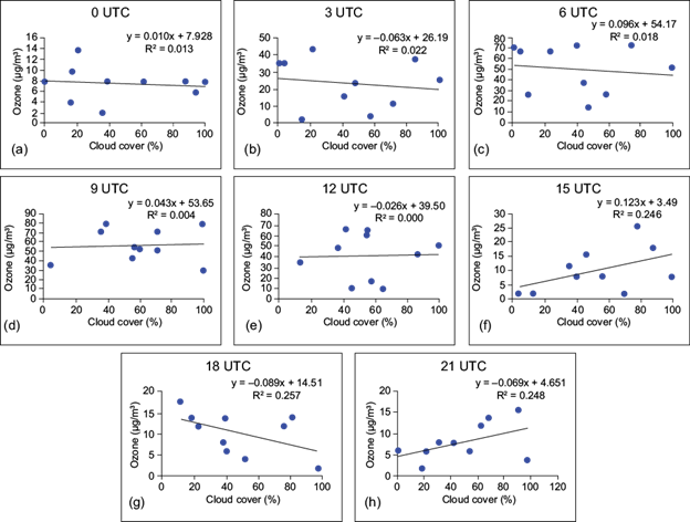
Fig. 9 Simple regression between surface ozone (µg m-3) and cloud coverage (%) at (a) 00 UTC, (b) 03 UTC, (c) 06 UTC, (d) 09 UTC, (e) 12 UTC, (f) 15 UTC, (g) 18 UTC, and (h) 21 UTC over site I.

Fig. 10 Simple regression between surface ozone (µg m-3) and cloud coverage (%) at (a) 00 UTC, (b) 03 UTC, (c) 06 UTC, (d) 09 UTC, (e) 12 UTC, (f) 15 UTC, (g) 18 UTC, and (h) 21 UTC over site II.
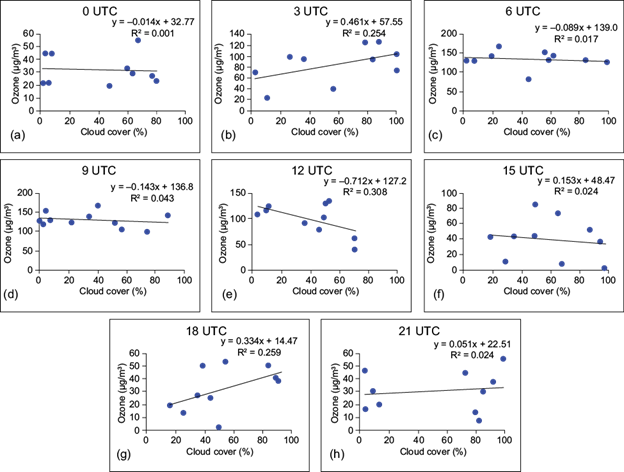
Fig. 11 Simple regression between surface ozone (µg m-3) and cloud coverage (%) at (a) 00 UTC, (b) 03 UTC, (c) 06 UTC, (d) 09 UTC, (e) 12 UTC, (f) 15 UTC, (g) 18 UTC, and (h) 21 UTC over Site III.
It appears from the figures that the coefficient of determination (R2) shows a very weak relationship between surface ozone and cloud cover. A similar result was found by Ghosh et al. (2015) over Kolkata, India. In the case of site I, negative relationships are observed at 03, 06 and 09 UTC, which indicates that after sunrise (daytime hours) the surface ozone concentration is regulated by the photo-oxidation of its precursors in presence of suitable meteorological factors. But during late afternoon and nighttime, cloud coverage does not play a significant role in controlling the surface ozone concentration.
At site III, the correlation between ozone and cloud cover is found to be negative at 06, 09 and 12 UTC. This indicates that the amount of surface ozone is driven by photochemical production during daytime as higher cloud coverage leads to lesser amount of ozone at the surface. But at night the concentration of surface ozone is a complex function of concentration of precursors, boundary layer characteristics and other meteorological factors. Horizontal wind transport also plays a crucial role in either accumulation or dispersion of surface ozone at all the sites.
An inverse correlation with humidity is found in all the air pollutants under consideration. Significant negative correlation of humidity is observed with concentration of PM10 (r = -0.514 and p = 0.004) and CO (r = -0.672 and p < 0.0001). This inverse relationship between humidity and PM10 is due to the effect of humidity on coalescence and the settling of fine suspended particles. The lifetime of the PM in ambient air increases in low humidity, resulting in higher concentration of PM10 in the atmosphere. Temperature is found to hold a positive correlation with SO2, NO2, NH3, CO and PM10. A positive relationship of ambient NH3 with temperature can be supported with by the fact that a rise in temperature increases evaporation of ammonia from PM and other sources present in the urban areas. This observation is further corroborated by the work of Perrino et al. (2002). All air pollutants hold an inverse relation with wind speed, which has a significant negative correlation with SO2 (r = -0.526 and p = 0.003), NO2 (r = -0.468 and p = 0.009), PM10 (r = -0.524 and p = 0.003) and CO (r = -0.524 and p = 0.003). High wind speed helps in the dispersion and dilution of air pollutants thereby reducing the pollution load near the earth’s surface.
3.3 Multivariate statistical analysis
Factors generated by multivariate statistical analysis give an insight into the main anthropogenic processes (industrial activities and vehicular emissions) that affect the concentration of different criteria pollutants in the ambient atmosphere. Principal component analysis on the composite data set has resulted in factors D1 and D2 (with eigen value > 1) that explain percentage of variability of data. Table III shows the loading of each variable within two selected factors. Factor 1 (D1) shows that loading of PM 10, SO2, CO, O3 and NO2 can be partially attributed to industrial emission.
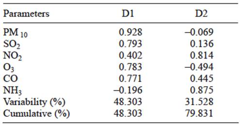
Although O3 is not directly emitted by nearby industries, the high concentrations of precursor gases emitted by these industries (along with suitable meteorological conditions) produce O3 (a secondary pollutant). Factor 2 (D2) shows a higher loading of NO2 and NH3 along with moderate loading of CO resulting from vehicular emissions.
3.4 Air quality index
Site-specific statistical summaries of air pollutants and AQIs are given in Table IV.

The site-specific statistical summary of air pollutants also supports the abundance of vehicular emissions (i.e., NO2, NH3 and CO) and industrial emissions (i.e., PM10, SO2, NO2 and CO) in the ambient atmosphere of sites I and III, respectively. AQI calculations (Mudri, 1990) show that site II (residential area) is clean (AQI = 22.69). Both site I (traffic congested area) and site III (industrial area) are found to fall in a moderately polluted category, though the latter is more polluted than site I.
4. Conclusion
The present study focuses on the variation of different air pollutants (PM10, SO2, CO, O3, NH3 and NO2), meteorological parameters (temperature, humidity, cloud cover, wind speed and wind direction) and PBL characteristics (height and vertical mixing coefficient) in the ambient atmosphere of three different sites in Durgapur, an urban region in eastern India. The major conclusions are given below:
High ground level ozone is found in a residential area (site II). Backward trajectory simulations suggest the occurrence of long-range transport of ozone. Moreover, air masses containing precursor pollutants also produce ozone as they travel. So, systematic assessment and control strategies should be made for residential areas since ozone has many adverse effects on human health. The calculation of AQIs for the three different sites show that sites I (area with high vehicular density) and III (industrial site) are moderately polluted with AQIs = 53.85 and 71.68, respectively, while site II (a residential area) is clean (AQI = 22.69).
Meteorological variables and boundary layer characteristics strongly influence the chemistry and dispersion of pollutants in the PBL. This work has identified the major pollutant sources over the three different sites and presents an idea of prevailing air quality status of different regions of this urban area .
The creation of comprehensive emission inventories of this urban area will further help to identify specific pollutant sources around the chosen sites, thereby helping in the formulation of more effective urban air quality management strategies.

