


 text new page (beta)
 English (pdf)
 Article in xml format
 Article references
 Send this article by e-mail
 Cited by SciELO
  Similars in
SciELO
Similars in
SciELO 
 Permalink
1. Introduction
The Indian Summer Monsoon (ISM), which is characterized by seasonal reversal of trade winds from northeast to southwest due to differential heating of the Indian landmass and neighboring oceans, is a major component of the tropical circulation. It contributes to more than 70% of the annual rainfall over India (Parthasarathy et al., 1994). Due to its large impact on Indian economy, the ISM has been an important topic of research for more than a century now. Numerous studies have been conducted to understand the mechanism and physical processes (i.e., large scale circulation processes) of the ISM (Shukla and Paolino, 1983; Shukla and Fennessy, 1994; Bhaskaran et al., 1996; Goswami et al., 1998; Webster et al., 1998; Lal et al., 2000; Zhou and Li, 2002; Mohanty et al., 2002, 2005; Kang et al., 2002; Rao et al., 2004; Singh et al., 2007; Raju et al., 2010; Zou and Zhou, 2013, 2014; Zhu, 2015; Almazroui et al., 2016). However, convection plays an important role in the development and maintenance of the ISM through the release of latent heat and vertical transport of heat, moisture and momentum (Ghosh et al., 1978; Kain, 1993; Zhu, 2015). A number of schemes have been developed over the years to parameterize the cumulus convection in large-scale numerical models, but none of the studies show a universal conceptual framework to parameterize convection. Thus, it is important to undertake a sensitivity study to have a suitable choice of convection scheme for a particular region.
A comparative study of different Kuo type of cumulus convection schemes (CCS) (Kuo, 1965, 1974) during different epochs (pre-onset, onset and break) of the Asian Summer Monsoon was conducted by Das et al. (1988), who inferred that the Kuo-Anthes scheme (Anthes, 1977) performs better in simulating heating, moistening and precipitation rate in a moderate convective regime. A similar kind of study was conducted by Alapaty et al. (1994) using the Naval Research Laboratory/North Carolina State University (NRL/NCSU) nested grid regional model with Kuo and Betts-Miller schemes (Betts, 1993) during an active monsoon period; they reported that different regional monsoon features are better simulated with the Kuo scheme. Das et al. (2001) performed a sensitivity study of ISM to CCS using the global spectral model of the National Centre of Medium Range Weather Forecasting (NCMWRF), India, considering three CCS, viz. the simplified Arakawa-Schubert scheme (SAS), the relaxed Arakawa-Schubert scheme (RAS), and the Kuo scheme. They concluded that SAS performed better in simulating the regional features of ISM. Das et al. (2002) carried out another sensitivity study using the above CCS to observe the skill of medium range forecast over the Indian region which corroborates their previous findings.
Dash et al. (2006) investigated the sensitivity of ISM on cumulus convection for a four-yr. period (1993-1996) using RegCM3 and concluded that the Grell scheme (Grell, 1993; Grell et al., 1994) performed better. Martínez et al. (2006) observed that the Grell scheme with Arakawa-Schubert closure is better in simulating summer precipitation in the Caribbean region using RegCM3. Venkata and Cox (2006) inferred that the Kain-Fritsch scheme (Kain, 1993) performed better than the Grell scheme in simulating monsoon depression using a mesoscale model (MM5). In a recent study, Sinha et al. (2013) showed that the MIT scheme (Emanuel, 1991) is a better choice for the simulation of ISM. These studies clearly indicate that the monsoon features are highly sensitive to the choice of CCS. Although, a number of studies on the ISM have been conducted using regional models, but mostly with the Biosphere-Atmosphere Transfer Scheme (BATS) (Dickinson et al., 1993). No study has been conducted so far using RegCM4 in combination with other land surface schemes present in the model (e.g, the Community Land Model [CLM] v. 3.5) for the seasonal simulation of ISM.
In this study an attempt is made to test the sensitivity of the ISM simulation to some of the CCS that have not been considered in earlier studies. The following section contains three subsections in which the model is described, numerical experiments are conducted and datasets are used. Results and discussions are presented in Section 3, followed by a conclusion in Section 4.
2. Model description, experimental design and datasets used
2.1 Model description
The regional climate model (RegCM4, version 4.1.1), which is developed by the Abdus Salam International Center for Theoretical Physics (ICTP, Italy), is an evolution of RegCM3 with inclusion of some improved physical parameterization schemes. Its dynamical core is, as its previous version (Pal et al., 2007) a hydrostatic, primitive equation model which has a terrain-following sigma coordinate in the vertical. RegCM4 consists of multiple state-of-the-art physics options. Radiative transfer calculations follow the radiative transfer scheme of the global model CCM3 (Kiehl et al., 1996). Along with the planetary boundary layer (PBL) scheme proposed by Holtslag et al. (1990) and used in RegCM3, a new PBL scheme developed by the University of Washington (Bretherton et al., 2004) is implemented in RegCM4. The model also includes parameterization schemes for ocean fluxes, interactive aerosol schemes and interactive lake models.
In RegCM3, land surface processes were described using BATS (Dickinson et al., 1993). In addition, CLM3.5 (Tawfik and Steiner, 2011), developed by the National Center for Atmospheric Research (NCAR) is coupled with RegCM4 to improve the representation of land surface processes. CLM has the best capability to represent various land surface process like snow and soil layers, land surface heterogeneity, land cover types and vegetation fraction (Steiner et al., 2005). A detailed description of CLM3.5 implemented in RegCM4 is presented in Steiner et al. (2009) and Collins et al. (2006).
In the RegCM4 modeling framework, precipitation is classified broadly into two categories, viz. non-convective scale (grid-scale) and convective (sub-grid scale). The former, also known as large/resolved scale precipitation is derived using the sub-grid explicit moisture scheme (SUBEX; Pal et al., 2000) while the later (sub-grid scale) is explained using different CCS mentioned below. The SUBEX scheme accounts for the sub-grid variability in clouds by linking the average relative humidity of a grid cell to the cloud fraction and cloud water, whereas the precipitation produced by a CCS illustrates the effects of sub-grid scale convective clouds.
There are three major CCS available in RegCM4, viz. MIT (Emanuel, 1991), Grell (Grell, 1993; Grell et al., 1994), Kuo (Anthes, 1977). A Major improvement in RegCM4 is the option of choosing different CCS over land and ocean (mixed scheme), instead of using a single CCS over the whole model domain. The reason is the limited performance of CCS over land and ocean (Giorgi et al., 2012); therefore, in addition to the three main CCS, the model has two mixed convection schemes: Grell over land and MIT over ocean (GL_MO) and Grell over ocean and MIT over land (GO_ML).
In the Kuo scheme (Anthes, 1977), the convection is activated when the moisture convergence of a column exceeds a threshold value and vertical sounding is convectively unstable. A fraction of the moisture convergence moistens the column and the remaining forms precipitation. It is explicitly mentioned that the moisture convergence of an atmospheric column is computed considering the advective tendency of water vapor only. The latent heat due to condensation is distributed between the cloud top and bottom by a function that allocates the maximum heating to the upper portion of the cloud layer (Giorgi et al., 2011).
The second CCS option is the Grell scheme (Grell, 1993; Grell et al., 1994), which assumes that the convective cloud stabilizes the environment as fast as the non-convective cloud destabilizes it. It is a mass flux convection scheme that considers the cloud as a two steady-state circulation having an updraft and a penetrative downdraft. The updraft and downdraft are initiated at the level where the moist static energy is maximum and minimum, respectively. It works when a lifted air parcel in the updraft attains moist convection level. The mixing of cloudy and environmental air is possible except at the top and bottom of the circulation. The mass flux is assumed to be constant and no entrainment/detrainment is allowed through the cloud edges. The scheme is employed with a closure approximation such as the Arakawa and Schubert (Arakawa and Schubert, 1974; Grell et al., 1994) closure or the Fritsch and Chappell closure (Fritsch and Chappell, 1980).
The third CCS option is the MIT scheme (Emanuel, 1991; Emanuel and Zivkovic-Rothman, 1999), where it is assumed that the cloud mixing is highly episodic and inhomogeneous and convection is triggered when the level of neutral buoyancy is greater than the cloud base level. A part of the condensed moisture forms precipitation and the remaining part forms cloud between these two levels. The fraction of the total cloud base mass flux that mixes with the environment at each level is proportional to the change rate of undiluted buoyancy with altitude. A more detailed description of RegCM4 is available in Giorgi et al. (2012).
2.2 Experimental design
The configuration of the model used in the present study is given in Table I. The model domain ranges from 30-120º E, 15º S-45º N with 30-km horizontal resolution and 23 vertical levels (Fig. 1). The initial and lateral boundary conditions are provided by global reanalysis datasets. Similar to the other regional model, RegCM4 is employed with a buffer zone of 12 grid points inside the lateral boundary (Wang et al., 2003; Giorgi et al., 2011). Different prognostic variables of the model, such as wind components, temperature, water vapor, etc., are nudged to the reanalysis data with an exponential nudging technique. The polygon inside the model domain (Fig. 1) represents the buffer zone selected for this study.

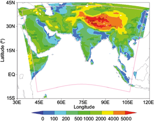
Fig. 1 Model domain and topography of the study region (in meters) along with buffer zone of the model.
The model is integrated from 00:00 UTC on May 1 to 18:00 UTC on September 30 for seasonal simulations of the ISM in 2007, 2008, and 2009. First, one month (May) is considered as the model spin-up period based on previous studies (e.g., Dash et al., 2006; Tchotchou and Kamga, 2010; Sinha et al., 2013; Zou et al., 2014; Tiwari et al., 2015); then, the simulation for the period June-September is considered for the analysis. Although spin-ups of regional models vary in the range of 10 days to one month (Wang et. al, 2003; Martínez et al., 2006; Zhong et al., 2006; Kang et al., 2014) and even longer for climate scale simulation, one month is sufficient for a seasonal scale (five months) simulation to achieve dynamical equilibrium of the model internal physics and lateral boundary conditions, as mentioned in the earlier literature. It is reported in an earlier study by Anthes et al. (1989) that regional models reach the equilibrium stage around 2-3 days. Five numerical experiments with five CCS (MIT, KUO, GRELL, GO_ML and GL_MO) for each of the three years (2007, 2008, 2009) are conducted in this study. The Indian Meteorological Department (IMD) provides a detailed report regarding different features of the monsoon, including the indian summer monsoon rainfall (ISMR) for the years 2007-2009 at http://www.imdpune.gov.in/Clim_Pred_LRF_New/Reports/Monsoon_Report/. As reported by the IMD, 2007 was an above-normal year with 105% of all India rainfall (long period average), 2008 was a normal year with 98% of all India rainfall, and 2009 was a deficit monsoon year with 77% of all India rainfall. The long period average rainfall is the average of the ISM precipitation for 1951-2000; it provides an opportunity to investigate the performance of RegCM4 in these three contrasting monsoon years.
2.3 Datasets used
The meteorological parameters for the initial and boundary conditions of the model were derived from the NCEP/NCAR reanalysis (Kalnay et al., 1996) at 2.5º × 2.5º resolution. The geophysical parameters, viz. topography and land use, are obtained from United States Geological Survey (USGS) global data at 10 min resolution. Sea surface temperature (SST) for the model initial condition is taken from NOAA optimum interpolation (OI) global data at 1º × 1º resolution. Additional datasets including land cover, soil texture and color, leaf area index, etc., required for CLM, are obtained from http://clima-dods.ictp.it/data/regcm4/CLM/. Surface temperature and rainfall simulated by the model were validated with high resolution (0.5º × 0.5º) Climate Research Unit time series (CRU TS 3.22) datasets (Harris et al., 2014; Trenberth et al., 2014). Wind fields and different fluxes from the model simulation are compared with NCEP/NCAR datasets.
3. Results and discussion
The model-simulated results with different convection schemes are analyzed and presented to evaluate their performance in simulating important features of the monsoon and seasonal and monthly scale precipitation over India and its five homogeneous regions. At first, surface temperature is analyzed in reference to heat low, land-ocean temperature gradient and its spatial variation over the region in the monsoon season (section 3.1). Next, the monsoon circulation features in the three consecutive monsoon years are discussed in section 3.2. Rainfall distribution over India and its homogeneous regions is discussed in the subsequent section. The homogeneous regions considered for this study, viz. northwest India (NWI), west central India (WCI), central northeast India (CNEI), south peninsular India (SPI) and northeast India (NEI), are based on rainfall characteristics (Parthasarathy et al., 1994) (see Fig. 3). The model’s ability to capture surface temperature and rainfall is also evaluated by means of different statistics such as spatial correlation, standard deviation and root mean square error (RMSE) using the Taylor diagram (Taylor, 2001), which provides pictorial representation of these features in a single diagram and is successfully used in numerous studies (Ali et al., 2015; Almazroui et al., 2016).
3.1 Surface temperature
Figure 2 presents June-September (JJAS) averaged temperature (ºC) for the years 2007-2009 from model simulations using the MIT, GRELL, KUO, GO_ML and GL_MO schemes and the CRU dataset. It clearly indicates that the model using MIT, GO_ML and GL_MO (KUO and GRELL), produces higher (lower) surface temperatures in all of three years compared to the CRU dataset over the whole domain, except peninsular India. Heat low over northwest India and Pakistan is reasonably well simulated using MIT, GO_ML and GL_MO. It is also observed that heat low is elongated to eastern India in the simulation with the MIT scheme. Temperature at the center of the heat low is overestimated in all of the three CCS (it varies in the range of 33-35 ºC in the CRU observation, which is more than 35 ºC in the model simulation). The region of heat low has larger spatial extent in the model simulation using the MIT scheme. Although higher surface temperature is noticed in the three schemes, MIT shows slightly higher (2-3 ºC) temperature. The strength of the heat low as well as the temperature over Indian landmass is not well simulated using GRELL and KUO.

Fig. 2 JJAS averaged surface temperature (at 2 meter) for the year 2007, 2008, 2009 as obtained from model simulations and CRU dataset.
The bias (observation-model) in the model simulated JJAS averaged surface temperature is analyzed in all of these years. For brevity, a figure is not presented as a part of the manuscript. A warm bias is observed in the model simulation with MIT and two mixed schemes, viz. GO_ML and GL_MO over most part of the Indian landmass. Although the pattern of the bias is similar in all of these three schemes, the magnitude is higher in MIT. This result is consistent with many previous studies (Zou et al., 2014; Tiwary et al., 2015).
The temperature bias varying in the range of 1-5 ºC (even more in some regions) is observed over large areas in different parts of India (NWI, north India, Gangetic West Bengal and central India) using MIT except in peninsular India, where a slight cold bias (0.5-1 ºC) is observed. The temperature bias over the 4 regions using GO_ML and GL_MO (the mixed schemes) is found to be 0-3 and 0-2 ºC, respectively. A significant cold bias (more than 3 ºC) is observed in the simulation with KUO and GRELL. As a whole, the model using GL_MO reproduces the surface temperature better compared to MIT and GO_ML in each of the three years.
Biases in the model simulated surface temperature over different homogeneous regions (Fig. 3) of India using all the schemes (Table II) are analyzed to examine the model performance over different parts of India. It is clearly specified that the model shows a positive bias in the simulation with MIT in all the homogeneous regions except peninsular India in each of the three years. A significant negative bias is observed with KUO and GRELL over all of the homogeneous regions, with exception of 2008, when GRELL shows a slight warm bias over WCI. Although the signature of the positive/negative bias in the model simulated surface temperature over different regions varies form year to year, the detected magnitude of the bias is lower in GO_ML and GL_MO. No particular scheme has a better performance in all the regions. The model shows a better skill with GO_ML, GL_MO and MIT over NWI, CNEI SPI and NEI, respectively, irrespective of the years. Better performance is observed with GL_MO, GRELL and GO_ML in 2007, 2008 and 2009, respectively over WCI. Considering all the regions, the model performance is relatively better in the simulations with two mixed schemes, and specifically with GL_MO.
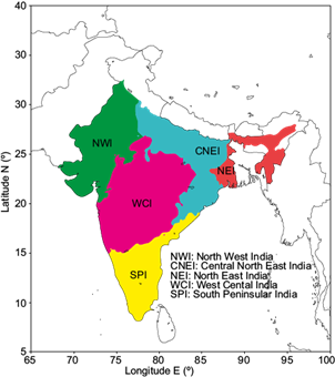
Fig. 3 Five homogeneous regions (Partahsarathi et al., 1994) over which performance of the convection schemes are evaluated.
Table II Scheme-wise bias of surface temperature during 2007-2009 over different homogeneous regions.
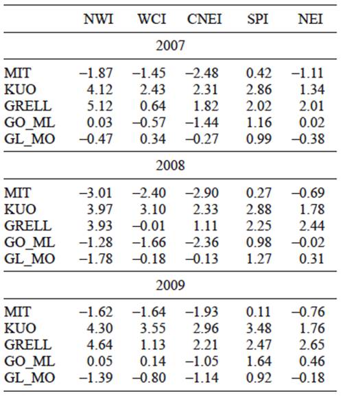
NWI: Northwest India; WCI: west central India; CNEI: central northeast India; SPI: south peninsular India; NEI: northeast India.
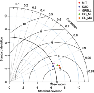
The Taylor diagram depicted in Figure 4 represents spatial correlation, standard deviation and RMSE between modeled and observed temperature (CRU). The design of the diagram considers the average of seasonal (JJAS) surface temperature for three years. It shows that the model performs reasonably well with all the CCS. The highest correlation (~0.97) and lowest RMSE (~2.1 ºC) are obtained using GL_MO, while the modeled standard deviation is almost equal to the observed one using KUO and GRELL. The other three schemes show a slightly higher standard deviation (7.5 ºC), which infers that spatial distribution and accuracy are better simulated by the model with GL_MO followed by MIT and GO_ML, with slightly higher variations than the CRU observation.
Seasonally averaged (JJAS) sensible heat flux (SHF) simulated by the model using different convection schemes along-with NCEP/NCAR datasets is presented in Figure 5. A higher SHF is noticed in the model simulation with MIT and the two mixed schemes specifically over central and northwest India. The highest SHF is noticed using MIT, which may lead to model simulation of higher surface temperature with those schemes. A lower magnitude of SHF over Indian landmass is observed in the simulation with KUO, indicating lower surface temperature with that scheme. This result is consistent with an earlier study by Nayak et al. (2017). Analyzing seasonally averaged fractional cloud cover (figure not shown), it is observed that the model produces lower values using MIT compared with the other schemes. This indicates that a larger amount of solar radiation reaches the land surface and increases the SHF, which results in higher surface temperature in the model simulation with MIT.
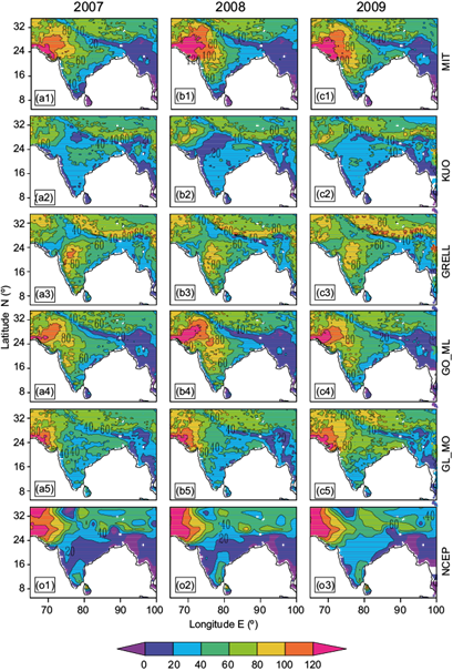
Fig. 5 JJAS averaged sensible heat flux (W/m2) for the year 2007, 2008, 2009 as obtained from model simulations and NCEP reanalysis dataset.
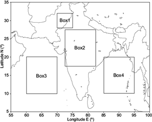
The model-simulated monthly mean surface temperature for JJAS (figure not shown) in 2009 (a draught year) shows a weaker heat low located over a smaller area. This is in agreement with the IMD monsoon report for that year. Dynamics of the monsoon circulation mostly depend upon the land ocean temperature gradient over the Indian subcontinent during the monsoon period. To analyze this aspect, four grid boxes (based on Mohanty et al., 2002) are introduced as shown in Figure 6, Box1 over NWI (70-75º E, 28-32º N), where the heat low dominates during monsoon season; Box2 over central India (72.5-82.5º E, 17.5-27.5º N); Box3 over the Arabian Sea (60-70º E, 10-20º N) near the east of Somalia coast, and Box4 over the Bay of Bengal (85-95º E, 10-20º N). The differences in the area averaged surface temperatures between these boxes in the month of May are computed and compared with NCEP/NCAR data due to non-availability of CRU temperature data over the oceanic region. The temperature differences between Box1 and Box3 in 2007 (a normal monsoon year) and 2009 (a deficit monsoon year) are 5.19 and 5.11º C, respectively, in the simulation using MIT, whereas in the NCEP/NCAR reanalysis datasets they are 3.27 and 3.28º C, respectively. This implies that the model is able to reproduce the temperature gradient for the two contrasting years better than NCEP datasets. The temperature difference between Box2 and Box4 in the simulation using MIT and NCEP data are 2.18º C, 5.2º C, respectively in 2007, and 4.44º C, 5.5º C, respectively in 2009, which clearly indicates that the temperature gradient between central India and the Bay of Bengal shows inverse relationship with that between NWI and the Arabian Sea in contrasting monsoon years.
3.2 Monsoon circulation
3.2.1 Low level winds (850 hPa)
Figure 7 presents the seasonal (JJAS) winds at 850 hPa computed from model simulations and NCEP/NCAR reanalysis for the years 2007-2009. The three columns of Figure 7 represent the simulation in three different years while the six rows correspond to five CCS and the reanalysis datasets. The model is able to simulate low-level circulation features such as the Somali jet stream, strong westerly winds over the Arabian Sea, the cross equatorial flow, the westerly flow over Indian landmass, etc., in all of the years with all of the schemes. It is also worth to mention that the performance of RegCM4 in simulating low-level circulation is comparatively better with MIT than with other schemes. Although the model underestimates the strength of the winds over both land and ocean in every CCS, it is lower in MIT followed by GO_ML and GL_MO. KUO and GRELL produce significantly weaker (5-8 m s-1) winds over the entire model domain.

Fig. 7 JJAS averaged lower level wind (at 850 hPa) for the year 2007, 2008 and 2009 as obtained from model simulations and NCEP/NCAR reanalysis. The colour shading represents the magnitude of the wind (m s-1) and the arrows are the direction.
In the year 2007, the strength of the Somali jet and cross equatorial flow are found to be 16 and 10 m s-1, respectively, in the simulations with MIT, while the same are found to be 18 and 10 m s-1 in the NCEP reanalysis data and in the range of 8-12 m s-1 in all other schemes. The westerly flow over the Arabian Sea and southern peninsular India simulated by the model is weaker except with MIT. The flow over the Bay of Bengal is also reasonably well simulated by the model with MIT (maximum strength is ~10 m s-1). Moreover, the area over which strong wind is simulated by the model agrees well with the reanalysis though the spatial extent differs.
The model exhibits similar performance in 2008 and 2009. However, the monthly average winds (figure not shown) for August and September 2009 show that the low-level wind is significantly weaker compared to that in 2007 in the simulation with MIT. The difference between model-simulated seasonal winds in 2007 and 2009 (figure not shown) shows that the strength of the Somali jet in 2009 is 2-3 m s-1 weaker than in 2007 in the simulation with MIT, GL_MO, and GO_ML. Another interesting fact to be mentioned here is that unlike the reanalysis datasets, RegCM4 with MIT could simulate stronger westerly winds over the Bay of Bengal in 2009 than in 2007 and 2008, which is consistent with the findings of Raju et al. (2010) and Mohanty et al. (2005). This indicates that the model with the above mentioned schemes could be able to simulate the differences in wind magnitudes during contrasting monsoon years. With GRELL and KUO, the model does not simulate this contrasting feature.
It is important to note that low-level winds in the RegCM4 simulation with all CCS is weaker compared to reanalysis data. In particular, the region of the south easterly flow before crossing the Equator shows smaller spatial coverage in the model simulation than in NCEP/NCAR data. This weaker wind flow favors a weaker Somali jet in the simulation, which may lead to less supply of moisture to the Indian landmass. Underestimation of low-level winds in the RegCM simulation is also observed and discussed in Sinha et al., 2013. In addition, a close inspection reveals that the circulation over central India shows an anti-cyclonic structure, which may hamper the moisture pulling mechanism from the neighboring ocean and lead to suppress the convective activity. This positive feedback between convective rainfall and low-level southwesterly winds is discussed in previous studies (Zou and Zhou, 2013; Zou et al., 2014). Overall, the model reproduces the low level-wind reasonably well with MIT compared to other schemes.
3.2.2 Upper level winds (850 hPa)
Seasonal winds at 200 hPa as obtained from model simulations and NCEP/NCAR reanalysis are shown in Figure 8. As mentioned in section 4.2.1, columns in Figure 8 represent the winds in three different years and rows depict the winds with five CCS and the reanalysis. Important upper level circulation features during ISM are the Tibetan anticyclone, the subtropical westerly jet (STWJ) and the tropical easterly jet (TEJ). Although the circulation pattern is well simulated by the model with all of the schemes, scheme-wise variation is noticed in terms of strength at the core of these wind jets, their respective position and spatial extent. As seen in the case of low level wind, RegCM4 shows better skill with MIT in simulating upper level circulation compared to other available CCS.
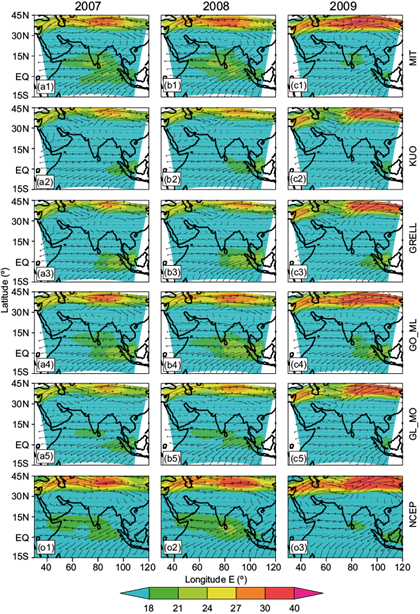
Fig. 8 JJAS averaged upper level wind (200hPa) for the year 2007, 2008, 2009 as obtained from model simulations and NCEP/NCAR reanalysis. The colour shading represents the magnitude of the wind (m s-1).
The location of the TEJ is well simulated by the model with MIT, though its strength is slightly overpredicted in all the years. TEJ is clearly observed from Thailand and Indonesia and is extended up to the east coast of South Africa covering the southern part of Indian landmass in the model simulation with MIT during normal monsoon years (2007, 2008).
The magnitude of the wind at the core of the TEJ in the simulation with MIT and NCEP data is about 20 m s-1. The strength of the TEJ is underpredicted and its position is moved eastward of its normal position (80º E, 5-10º N) in the simulation with GRELL and KUO. The model could be able to reproduce TEJ using GO_ML but fails in the simulation using GL_MO in all of the three years. It is interesting to note that the spatial extent of TEJ is less in 2009 (a deficit monsoon year) compared to 2007 (above normal year) and 2008 (normal year) in MIT, which agrees well with reanalysis data. Moreover, the strength of TEJ at the southern peak of Indian Peninsula is higher in 2007 and 2008 compared to 2009 in the model simulation using MIT, which is in good agreement with the reanalysis data. This infers that the model is able to simulate the contrasting monsoon features of upper level wind using MIT. These findings agree with Sinha et al., 2013.
The SWTJ is also reasonably well simulated by the model with all the schemes but slightly better with MIT. The STWJ is located to the north of the Himalaya (around 40º N) in all years. The magnitude at the core of STWJ in the simulation using MIT as well as reanalysis data is about 32 m s-1 but the core is more spatially extended in the model simulation. As noticed previously, in case of TEJ, the strength of the SWTJ is also significantly weaker in the simulations using other schemes. This clearly shows that the intensity of SWTJ is greater in deficit years (2009) than in normal or above normal years (2007 and 2008), which is in good agreement with Sinha et al., 2013. Unlike the reanalysis datasets, in the model simulation with MIT the center of the Tibetan anticyclone is prominently well positioned at about 30º N, 85º E. It is notably weaker and is not clearly visible in other CCS. The model was not able to show its shifting eastwards in 2009 as compared to 2007 and 2008 using MIT.
Considering overall performances, the characteristic features of the upper level wind as well as circulation are reasonably well simulated by the model with MIT.
3.3 Rainfall distribution
Rainfall is one of the most significant climatic parameters due to its huge societal impact. As reported in Almazroui et al. (2016), it is the most difficult-to-estimate parameter in the evaluation of a regional model due to its significant spatio-temporal variation, uncertainty and biases (Almazroui, 2013; Islam, 2009). Therefore, better simulation of rainfall using different CCS within a modeling framework remains always a challenge to climate researchers since its inception. In this section, model simulated rainfall using five CCS is analyzed and discussed.
Seasonal monsoon (JJAS) precipitation for the years 2007-2009, as obtained from the model simulations and CRU rainfall datasets, is presented in Figure 9. Rows in the figure represent the rainfall using different CCS and CRU rainfall, while columns show the rainfall in three different years. It clearly indicates that rainfall is underestimated by the model with all the schemes, particularly over central and NWI in all the years. The magnitude of this underestimation varies from scheme to scheme with reference to CRU rainfall. However, the rainfall is better simulated by the model with MIT and GO_ML compared to other CCS. It is noticed that the model with the above mentioned schemes correctly simulates the two rainfall maxima zones (Ratnam and Kumar, 2005): one over western Ghats and another over NEI and foothills of the Himalaya (Fig. 9), which is in good agreement with CRU data. Significant underestimation is observed in the simulation using GRELL and KUO, particularly over central India, where the simulated rainfall is less than 1 mm day-1.

Fig. 9 JJAS averaged rainfall for 2007, 2008 and 2009 as obtained from model simulations and CRU datasets in mm day-1.
Model biases (observation-model) in the simulation of seasonal rainfall for the above mentioned years are given in Figure 10. The model using all schemes shows a dry bias over large part of Indian landmass, Bangladesh, Myanmar and Thailand in all three years. The magnitude of the bias is comparatively lower in the simulation using MIT, GO_ML and GL_MO. The region over which significant dry bias (5 mm day-1) is noticed extends wider when KUO and GRELL are used. The model shows a wet bias of 0-5 mm day-1 using MIT and GO_ML over foot hills of the Himalaya and hilly regions of NEI. It is also noticed that with MIT and GO_ML the model shows a wet bias of 0-1 mm day-1 over some parts of the Indian peninsula, particularly in the rain shadow region of western Ghats except during 2007, when a dry bias is observed using GO_ML. Comparison of the simulations using MIT and GO_ML indicates that the dry bias is less over central India when GO_ML is used except in 2008.
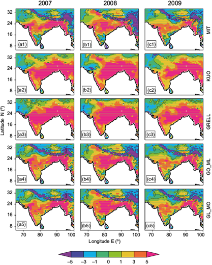
Fig. 10 Model bias for JJAS averaged rainfall for 2007, 2008 and 2009 as obtained from model simulations in mm day-1.
Similar biases are noticed in Nayak et al. (2017) and Maity et al. (2017). The simulation using GO_ML is more realistic in representing precipitation. The analysis of model bias over different homogeneous regions (Fig. 3) reveals underestimation of rainfall using all the schemes and in all the homogeneous zones (tables not shown). Only a slight overprediction is observed in 2008 in SPI and NEI, which indicates that model performance is comparatively better with MIT and GO_ML than with the other schemes except in NWI, where KUO performs better.
The difference in the model simulated rainfall between 2007 and 2009 (figure not shown) is analyzed to understand the fidelity of the model in producing yearly variations. It is observed that the model is able to simulate less rainfall in 2009 compared to 2007 over NWI, peninsular India, foothills of the Himalaya and NEI using MIT and GO_ML. The rainfall difference is minimal and not distinguishable in the model simulation using KUO and GRELL.
The monthly distribution (JJAS) of the ISMR for the years 2007-2009 from model simulations and CRU rainfall datasets is analyzed. For brevity, only the model results of 2007, along with CRU datasets are presented in Figure 11. Regardless of schemes and years, rainfall is underpredicted by the model using all the schemes, but is better represented with MIT and GO_ML. The model was unable to capture the monthly variation of rainfall in any of the years even with MIT and GO_ML. For example, in 2009, the model shows abundant rainfall in August and November, but according to the IMD report, rainfall in those months was significantly diminished (73% and 80%), which implies that the variation produced by the model is in contrast with the report of the IMD. Monthly rainfall is significantly underpredicted by the model with KUO and GRELL. The correlation coefficient and standard error in the monthly scale rainfall with CRU datasets shows that the model simulates more realistic rainfall with GO_ML.
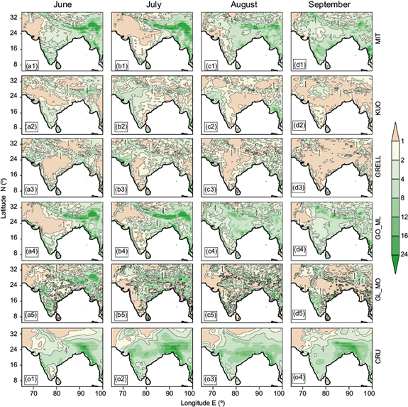
Fig. 11 Monthly rainfall as obtained from model simulations and CRU datasets for the year 2007 in mm day-1.
A Taylor diagram for three years average of seasonal (JJAS) rainfall, which is presented in Figure 12, shows that the distribution of rainfall is well simulated by the model using GO_ML and MIT compared to other schemes. These two schemes show a comparatively higher correlation (~ 0.55), lower RMSE (~4.4 mm day-1) and lower standard deviation (~ 4.5 mm day-1) than the other CCS. The performance of GO_ML is better than MIT as seen from the diagram, with slightly higher correlation and lower RMSE.
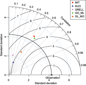
The correlation and RMSE of monthly rainfall is also analyzed (figure not shown). It is worth to mention that simulated rainfall is well distributed with KUO, particularly in June of 2007 and 2009. In a monthly scale, GO_ML shows better performance than MIT. The magnitude of rainfall is also better simulated by the model using GO_ML and MIT compared to other schemes. Overall, the distribution and magnitude of rainfall is better simulated by the model using GO_ML.
The ISMR shows considerable spatial variation, therefore it is important to investigate the capability of the model to simulate rainfall in different homogeneous regions. Model simulated mean seasonal (JJAS) rainfall along with CRU data, averaged for five homogeneous regions with the five convection schemes, is presented in the Figure 13. Rainfall over all the homogeneous zones is underestimated by the model using all schemes. Rainfall over WCI and CNEI is significantly underpredicted by the model except in 2009, when the model is able to simulate rainfall reasonably well using MIT and GO_ML over CNEI. Interestingly, the model performed consistently well with KUO over NWI. Figure 13 also indicates that seasonal rainfall is better simulated over different homogeneous regions in India using GO_ML and MIT compared to other schemes. Significant underprediction is observed with GRELL and KUO over all the homogeneous regions except NWI. The model shows less precipitation in 2009 compared to 2007 using MIT over NWI, WCI, NEI, SPI; the exception is CNEI, where it shows overprediction. Similarly, the simulation with GO_ML shows underprediction over NWI, WCI and CNEI and NEI and overprediction over SPI in 2007 and 2009.

The above discussion indicates that the model shows a dry bias using all schemes but exhibits better performance with MIT and GO_ML in simulating rainfall both in monthly and seasonal scales. Figure 14 represents model simulated seasonal average latent heat flux (LHF) with all schemes and NCEP data. It shows that lower LHF is simulated by the model with all schemes. A lower LHF may lead to less moisture availability at the surface resulting in a dry bias within the model simulation. It is also noticed from the figure that the simulated LHF is closer to NCEP data over foot hills of the Himalaya and NWI. Higher LHF enhances the rainfall simulation, which results in a wet bias over those regions using MIT and GO_ML. The dry bias in the model over central India using MIT and GO_ML may be due to the lower LHF observed over the region. For the other schemes (KUO and GRELL) LHF is significantly lower as may be noticed in Figure 14 and could be the cause of the dry bias.

4. Summary
This study discusses the relevant features of ISM, viz. heat low, Somali jet and southwesterly wind, subtropical westerly, tropical easterly jet, etc., through a sensitivity analysis of RegCM4 simulation using five convection schemes. The model shows a positive temperature bias in the simulation of surface temperature with the MIT, GO_ML and GL_MO schemes, and a cold bias using the KUO and GRELL schemes. The spatial distribution and magnitude of surface temperature is slightly better simulated with GL_MO compared to the other convection schemes. The seasonal mean circulation, as well as the change in strength of circulation in the contrasting monsoon years (2007 and 2009), are well simulated by the model with MIT. Seasonal and monthly mean rainfall are underestimated by the model with all convection schemes and show a wet bias in the foothills of the Himalayas and NEI. It is noticed that GO_ML shows better skill in simulating monsoon rainfall.
The results indicate that the best CCS option varies from parameter to parameter and no particular convection scheme shows better performance in simulating all parameters (temperature, winds and rainfall). As seen before, surface temperature and rainfall amount are well reproduced by the model with GL_MO and GO_ML, while low level and upper level circulation are better simulated with MIT only. A variation in model performance is also noticed when the simulation over different homogeneous zones is taken into consideration. It is observed that the performance of the model with MIT is slightly inferior to GL_MO and GO_ML but substantially superior to the remaining CCS in simulating surface temperature and rainfall. As mentioned earlier, higher (lower) surface temperature (rainfall) over central and NWI in the model simulation with MIT may be due to higher (lower) sensitivity heat flux (LHF) noticed over those regions. Therefore, as far as detection of a single CCS is concerned, MIT may be considered as the most suitable for simulating the ISM.

