1. Introduction

Vortex shedding occurs downstream of the Hong Kong International Airport in certain meteorological conditions. Such vortices can be hazardous to aircraft landing or departing from that airport. ^{Chan (2012}) documents the environmental flow associated with, and a numerical simulation of, a series of vortices shed from the Nei Lak Shan Mountain southwest of the Hong Kong International Airport (HKIA) on April 11, 2011. In that analysis, Doppler Light Detection And Ranging (LIDAR) conical scan data were used only. This paper extends the previous study by considering surface observations and examining the LIDAR data in greater depth to enable a more detailed analysis of the vortex structure.

The perturbation of the ambient environmental flow by the mountain on this day measured by the southern airport LIDAR is illustrated in Figure 1. A channel of weakened southeasterly flow is located downstream of the elevated terrain south of the airport. Elongated swaths of cyclonic and anticyclonic azimuthal shears, as evidenced by differences in Doppler velocity at constant range from the LIDAR, are located on the northern and southern peripheries of the wake channel (along dashed lines in Fig. 1), with isolated areas of enhanced shear located within them. This flow pattern is qualitatively consistent with past modeling studies of weakened environmental flow and wake vortices produced downstream of isolated terrain maxima (e.g., ^{Schar and Smith, 1993a}, ^b; ^{Sun and Chern, 1994}; ^{Schar and Durran, 1997}; ^{Young and Zawislak, 2006}). However, there are only a few detailed observational studies of such wake flow in the literature.

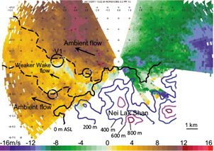
Fig 1 Single-Doppler velocity field from the 3.2° LIDAR scan at 13:22:34 UTC. Terrain contours on Lantau Island are shown in 200 m increments (starting at sea level). The approximate channel of weakened wake flow is outlined in dashed lines. The position of V1 is shown with a large black ring. Two smaller transient areas of locally enhanced cyclonic and anticyclonic azimuthal shear on either edge of the mountain wake flow are shown with thin black rings. North is up. 

This paper documents the kinematic structure of prominent vortices shed downstream of Lantau Island within this flow regime using a combination of surface weather buoy, LIDAR observations, and LIDAR-derived ground-based velocity track displays (GBVTD; ^{Lee et al., 1999}). The vortices were not in a geometrically suitable location for a dual-Doppler wind retrieval using the two airport LIDARs. The LIDAR used in the current study has a temporal resolution of ~90 s, is gated at 105 m and has a 2.0º beam width. Sweeps are at 3.2º and 6.0º elevations, which are based on the elevation angles of the arriving and departing aircraft respectively. Vortices typically are about 5 km in range from the LIDAR, yielding a spatial resolution of approximately 170 m in the horizontal and 260 masl in the vertical. The lowest LIDAR sweep collects data at approximately 260 masl in the vicinity of the vortices.

2. Characteristics of vortices shedding from the mountain

From approximately 13:00 until 14:00 UTC, observations from the southern runway LIDAR at HKIA depicted vortices shedding off the Nei Lak Shan Mountain traveling toward the northwest. Although several transient enhancements of azimuthal shear are located at the periphery of the wake flow of the island during this shedding event, three prominent rotating vortices (hereafter V1, V2, and V3) were observed by the LIDARs along the northern interface between the wake channel and environmental flow. The Doppler velocity couplets (regions of adjacent inbound and outbound Doppler velocities) for each vortex are evident in the lowest elevation angle sweep of the LIDAR from approximately 13:07-13:27 UTC for V1, 13:27-13:39 UTC for V2, and 13:35-13:44 UTC for V3. Figure 2 illustrates the observed tracks of the vortices relative to the airport, Lantau Island, and surface weather buoys. All three vortices travelled northwestward over water southwest of the airport. The path length and duration of V1 were nearly twice those of V2 or V3. The peak tangential velocities for each of the vortices, estimated as half of the peak azimuthal wind shear calculated from the difference between inbound and outbound Doppler velocities (ΔV) divided by 2 (i.e., ΔV/2) in the lowest LIDAR scan, are similar in magnitude, between 7 and 8 m s^-1 (Fig. 3). The velocity profiles for the three vortices are shown in Figures 3b-d. The evolution of velocity profiles of the first vortex is given in Figure 3b. Average core diameter of the vortices, estimated by measuring the distance between peak inbound and outbound LIDAR velocity extrema, is approximately 1000 m. Figure 4 shows LIDAR imagery of the three vortices at the approximate time of peak LIDAR-estimated tangential velocity for each. There is no clear correspondence between time tendencies of LIDAR-estimated core size and tangential velocity, nor with height across all vortices. More details of the three-dimensional structure of each vortex are presented in the GBVTD analyses.

Fig 2 Positions of three weather buoys, WB1, WB2, and WB5 (cyan markers) and LIDAR-estimated tracks of the three vortices, V1, V2, and V3 (red, green, and yellow dots, respectively). The first and last observed times of each vortex as well as select times when V1 is located within 1 km of WB5 are labeled along each track. Polynomial fits to the V1 and V2 tracks used to parameterize their positions in idealized axisymmetric vortex models are shown as red and green lines, respectively. North is up. LIDAR is located by a blue square. 

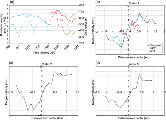
Fig 3 (a) Rotational velocity (solid lines) and core radius (dashed lines) measured in the lowest LIDAR elevation angle sweep for V1 (blue), V2 (red), and V3 (green). The Doppler velocity against the distance from the centers for V1, V2 and V3 are given in (b), (c) and (d), respectively. The time evolution of the velocity profile of V1 is shown in (b). 

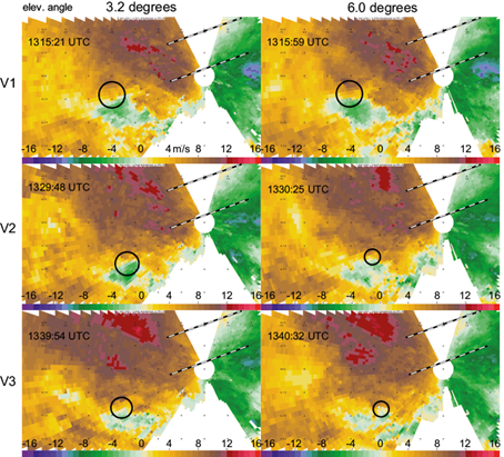
Fig 4 Radial velocities (m s^-1) of V1 (top row), V2 (middle row), and V3 (bottom row), measured by the southern airport LIDAR at 3.2º (left column) and 6.0º (right column) elevation angles. Positions of the vortices are indicated with rings. Images are shown at the time when the vortices have the strongest observed peak inbound and outbound radar velocity differential. The black lines depict the locations of the airport runways. 

3. Surface observations

Observations from three weather buoys (WB1, WB2, and WB5) located southwest of the airport were examined to determine if winds associated with the vortices were present near the surface. LIDAR-measured ground-relative positions of the three vortices indicate that the core flow of V1 passed almost directly over WB5 and that the edge of the core flow may have grazed WB2 (Fig. 2). Although V2 and V3 were located at a slightly farther distance from WB2 and WB5, it is possible that the outer part of their core flows may have passed near these buoys. The core flow regions of all three vortices were located comparatively far from WB1. Further focus is placed on analyzing the observations collected by WB5 because of its close proximity to the path of the central core flow region of V1 and its close proximity of the edges of the core flow regions of V2 and V3.

There appears to be a signal of the passage of V1 in the instantaneous wind speed and direction data (0.1 Hz sampling at z = 7 m ASL) at WB5 (Fig. 5). A 120º shift in the wind direction occurs as the core of V1 passes, returning to nearly its original direction after passage. The WB5 wind speed data oscillates with a magnitude of ~6 m s^-1 during V1 core passage.

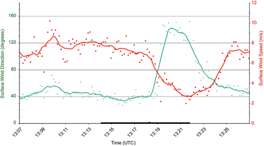
Fig 5 Surface wind speed and direction observations collected at WB5 as V1 passes. The observations (collected a 1-s frequency) are shown every 10 s. The period when the center of V1 (measured at the lowest LIDAR level) is estimated to be within 1 km of WB5 is illustrated with a black line. The ‘V1’ label along the line indicates the approximate time when the estimated center of the vortex is the closest to WB5. 

For independent verification that the observed surface wind anomalies are consistent with the influence of the passing vortices, assumed tangential wind profiles as a function of radial distance from the axis of rotation (Vtan) from V1 and V2 are modeled using a ^{Burgers-Rott idealized axisymmetric vortex (Burgers, 1948}; ^{Rott, 1958}).

(1)

In this model, Γ is circulation in the vortex, a is radial convergence, and ν is viscosity. This expression simplifies to (^{Wood and Brown, 2011}),

(2)

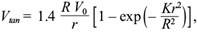
where r is the radial distance from the axis of rotation, V ₀ is the maximum tangential velocity of the vortex (ΔV/2), R is the core radius at which V ₀ occurs, and K is a shape parameter. Parameters V ₀ and R for V1 and V2 are calculated from LIDAR measurements at the lowest sweep (z ~260 masl), V ₀ varies in time for each vortex and R is set equal to the mean core radius of each, which is 480 m (R is constant rather than varying in time owing to uncertainties in its measurement using LIDAR observations). K = 1.2564, a theoretical value calculated by ^{Davies-Jones and Wood (2006}) and adopted in ^{Wood and Brown (2011)}. Observations of vortex position and V ₀ are interpolated via a polynomial fit at 10-s intervals to facilitate calculations at time steps between LIDAR sweeps (the polynomial fit to the positions of V1 and V2 used in these models are shown in Fig. 2).

Using the distance between WB5 and each of V1 and V2, the tangential winds from the modeled vortices are combined via vector addition to simulate the wind trace at WB5 resulting from the influence of both at each time (Fig. 6). The environmental wind speed was chosen as the mean vortex motion (4 m s^-1, assuming that the vortices were traveling with the mean flow in which they were embedded) and the environmental direction was chosen from the WB5 trace (55º). There is a large amount of uncertainty in the environmental wind measurements near the surface in this area owing to heterogeneous flow associated with the terrain, wake flow, and other areas of cyclonic shear neighboring V1-V3. Additional Burgers-Rott vortex models are composed with environmental wind speeds and directions modified by ±20% (LIDAR-estimated V ₀ and R also are modified by 20%) to crudely evaluate some of this uncertainty (shaded regions in Fig. 6). Finally, another Burgers-Rott vortex model that estimates V ₀ near the surface for both vortices to be ~50% of that at the lowest LIDAR level, R ~ 700 m, and the environmental wind speed and direction to be 7 m s^-1 and 55º (these values are based on an estimate of ΔV/2 ~3-4 m s^-1 and the distance across the peak wind shift during V1 passage, and the wind prior to the passage of V1, each directly using the WB5 wind observations) also is shown in Fig. 6 (purple and blue lines). The ensemble of these simulated wind traces (summarized in Table I) is intended to represent some of the uncertainty present in comparing them to the WB5 observations near the surface using mostly independent LIDAR estimates of vortex and environmental wind properties to model them.

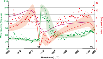
Fig 6 Comparison of WB5 wind speed and direction observations (dots) and those simulated at WB5 using Burgers-Rott vortex models of V1 and V2, each based on measurements of V ₀ and R from the lowest LIDAR level (red and green lines). Red and green shaded regions represent the area on the plot occupied by simulated wind traces from Burger-Rott vortex models that use V ₀ , R, and environmental winds that vary ±20% from those used to make the red and green lines. Another trace of wind speed (purple) and direction (blue) using a Burgers-Rott profile that assumes: R = 700 m, V ₀ that is 50% of that at the lowest LIDAR level, and environmental wind speed of 7 m s^-1 (each consistent with WB5 observations) also is shown. Parameters for each of these plots are summarized in Table I. The periods when the centers of V1 and V2 (measured at the lowest LIDAR level) are estimated to be within 1 km of WB5 are illustrated with black lines. The ‘V1’ and ‘V2’ labels along these lines indicate the times when the centers of the vortices are the closest to WB5. 

Table I Summary of the Burgers-Rott vortex mode parameters illustrated in Figure 6. 

Overall, the wind speed and directional changes observed at WB5 are qualitatively similar to those predicted by the vortex models which are based on the LIDAR observations collected from a few hundred meters above (Fig 6), suggesting that wind perturbations from the vortices were present near the surface. The LIDAR-based models underpredict the near-surface wind speed at WB5 during the initial approach of the core of V1 (before 13:15 UTC) and after V1 passes (after 13:24 UTC). However, the simulated wind direction traces match quite well with WB5 observations. The wind traces simulated using V ₀ and R estimated directly from WB5 observations (purple and blue lines in Fig. 6) appear to under-predict the wind speed and direction shifts observed at WB5 during the core passage of V1, but match observations much more closely before and afterward. Considering the fit of all of these simulated wind traces to WB5 observations, it seems likely that wind perturbations associated with both of these vortices were present near the surface, below the lowest LIDAR observations, and that the strength and radius of the surface vortices can be estimated using the parameters of a Burgers-Rott vortex model.

The influence of V1 may also be evident in the near-surface pressure observations at WB5. Figure 7 compares the WB5 near-surface air pressure trace (with the mean pressure trend during the observation period, 0.006 hPa s^-1, removed to increase the sensitivity of detecting pressure tendencies occurring on the time and spatial scales of the vortices) to cyclostrophic pressure retrieval,

Fig 7 Comparison of the WB5 pressure trace (with the environmental pressure trend removed; dots) and retrieved cyclostrophic pressure traces associated with the Burgers-Rott vortex model illustrated with bold red and green lines in Figure 6 (red line). The period when the center of V1 (measured at the lowest LIDAR level) is estimated to be within 1-km of WB5 is illustrated with black line. The ‘V1’ label along the line indicates the approximate time when the center of the vortex is the closest to WB5. The dashed black line is for a modified Rankin vortex with V ₀ = 9 m s^-1, R0 = 450 m (and α = 0.7 and ρ = 1.25) as in ^{Inoue, et al 2011}. 

(3)

where Vtan is the tangential wind profile from the Burgers-Rott vortex model (described above), r is distance from the central axis of rotation, and Δr is the difference between the distance at neighboring observation times (Δr varies with time depending on observed vortex position and is ~100 m on average using the polynomial tracks with 10-s time steps described above). The environmental pressure is determined empirically to be 1008.7 hPa using the detrended WB5 pressure observations from several minutes prior to V1 passage. There appears to be a brief 0.5 hPa drop in the detrended WB5 surface pressure data during the passage of V1, minimized at approximately 13:18 UTC. This observed pressure minimum occurs simultaneously with the pressure minimum of the LIDAR-based cyclostrophic model retrieval, differing by approximately 0.2 hPa. Given the small magnitude and short duration of the apparent observed pressure drop, it is not entirely clear if this is associated with a vortex passage. However, the simultaneous observed and modeled pressure traces are perhaps compelling evidence that a subtle pressure drop associated with V1 was observed near the surface. Fitting of the pressure deficit curve is given in Figure 7 following the method of ^{Inoue et al. (2011}).

4. GBVTD analysis

To retrieve a three-dimensional vortex structure from the single-Doppler LIDAR scans, GBVTD analyses were conducted using the 3.2º and 6º elevation angle sweeps during three different time periods: 13:06:41-13:26:54 for V1, 13:26:54-13:38:27 for V2, and 13:35:34-13:44:41 for V3 (Figs. 8, 9). Following a similar approach to that of ^{Lee and Wurman (2005}), ^{Kosiba et al. (2008}, ²⁰¹⁴), ^{Kosiba and Wurman (2010}, ²⁰¹³) and ^{Wurman et al. (2013)} integration of surface weather buoys data with GBVTD wind retrievals derived from LIDAR data provided a time history of the three-dimensional wind fields of three vortices shedding from the mountain.

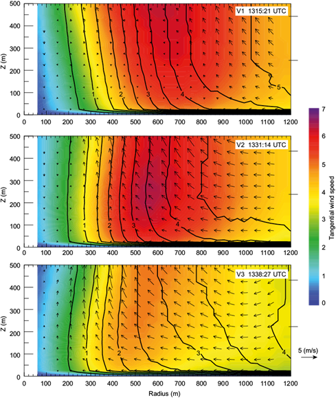
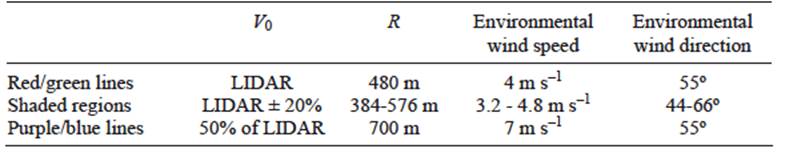
Fig 8 Axisymmetric vertical profiles (radial-vertical plane) of tangential velocity (shaded), angular momentum (contours; × 1000 m2 s^-1) and flow in the radial-vertical plane (vectors) at the time representative of the strongest tangential wind observed with LIDAR for V1 (top), V2 (middle), and V3 (bottom). White dashed lines are the approximate altitudes at which the 3.2º and 6.0º LIDAR elevation angle scans sweep through each vortex. A wind vector of 5 m s-1 is indicated. 

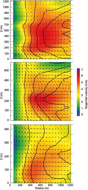
Fig 9 Hovmoller diagrams of GBVTD-retrieved axisymmetric tangential velocity (shaded), angular momentum (contours; × 1000 m2 s^-1), and flow in the radial-vertical plane (vectors) at z = 250 masl during the lifecycles of V1 (top), V2 (middle), and V3 (bottom). A wind vector of 5 m s^-1 is indicated. 

Before the GBVTD technique was applied, the LIDAR data were interpolated to a Cartesian grid using a ^{Barnes (1964}) scheme with horizontal and vertical smoothing parameters of 0.0225 and 0.0625 km², respectively, and a grid spacing of 30 m in the horizontal and 25 m in the vertical (this fine grid spacing, considerably finer than the data resolution, was used to improve plot quality). The GBVTD analysis was then conducted at radial increments of 30 m out to a distance of 1200 m from the vertical axis of rotation. Sensitivity tests revealed that the results were relatively insensitive to the grid spacing and Barnes smoothing parameters, with the exception of the magnitude of the tangential velocity, which was reduced slightly by larger smoothing. However, the spatial structure of the wind field was relatively unaffected. The winds are assumed to weaken logarithmically to zero at the surface below the lowest LIDAR level using a surface roughness length of 0.0002 m, a value consistent with an ocean surface (^{Stull, 1988}). This choice results in GBVTD-retrieved tangential winds for V1 at z = 7 masl that are similar in magnitude with those measured by WB5.

GBVTD-retrieved tangential velocity at the time of greatest vortex intensity increases with height in V1 and V3 (Fig. 8). However, the maximum tangential velocity in V2 is located at approximately z = 260 masl. The secondary circulation (flow in a radial-vertical plane) of V1 differs from that of V2 and V3. Inward (toward the axis of rotation) and upward flows are evident at all heights outside of the tangential velocity maximum of V1 (r ~ 650 m) and relatively weak radial-vertical flow is present inside of it. In contrast, radial inflow and updraft are present inside of the radii of maximum tangential wind for V2 and V3 (except nearly zero flow near the central vertical axis); therefore, relatively weak radial and vertical flow is confined to smaller radii for V2 and V3 than it is for V1. Although the radius of maximum GBVTD-retrieved tangential velocity is approximately 100 m larger for V1 than for V2 or V3, this difference is smaller than the difference between the smallest radius containing inward and upward flow, suggesting a slightly different secondary circulation pattern for V1 than for V2 and V3.

Peak tangential velocity at the height of the lowest LIDAR level ( 250 m) for each vortex (Fig. 9) is approximately 6 m s^-1 (although slightly smaller for V3), slightly less than observed using the raw LIDAR observations. These differences (Fig. 10) are due to the smoothing performed during the GBVTD retrieval. The GBVTD analysis retrieves either inward or weak radial flow and either updraft or weak vertical flow at the height of the lowest LIDAR scan at most times throughout the lifecycles of all three vortices. Relatively strong radial inflow and upward motion early in the lifecycle of V1 (e.g., before 13:11 UTC) occurs at all radii and contemporaneously with increasing angular momentum. This trend is possibly consistent with the inward advection of angular momentum resulting in the strongest GBVTD-retrieved tangential velocities associated with V1 between 13:12-13:17 UTC. Angular momentum and tangential velocity weaken after 13:17 UTC, concurrent with weak radial and vertical flow. Radial inflow and updraft are present throughout the entire lifecycles of V2 and V3, albeit radial and vertical flow weakens at r < 400 m during the period of peak tangential velocity of V2.

Fig. 10 Difference between the raw Doppler velocity measurements and the GBVTD analysis. 

Observations collected by WB5 during the passage of V1 suggest that the tangential velocity measured at 7 masl is 3-4 m s^-1, approximately half of that observed in the lowest LIDAR scan. Therefore, the majority of the logarithmic decay in tangential wind speed occurs in the lowest few meters above the surface. However, without having wind observations between the sea surface and the near-surface measurement height at WB5, and having very few observations below the lowest LIDAR level, the accuracy of the GBVTD-retrieved wind profile below z ~ 250 maslL cannot be confirmed and caution must be exercised when attempting to draw any conclusions about vortex properties in this vertical layer.

5. Summary

A variety of surface, LIDAR, and GBVTD-retrieved wind and pressure fields are used to examine the core-flow structure of three prominent vortices shed along the periphery of the wake of Nei Lak Shan Mountain when southeasterly flow impinged upon it on April 11, 2011. Measured at the level of the lowest LIDAR scan (approximately 260 masl), the average core flow of each vortex was approximately 1 km wide with an overall average peak tangential velocity of approximately 7.5 m s^-1. Although previous investigations of weather buoy data located southwest of the airport suggested no evidence of a surface wind pattern associated with the vortices, further examination indicates that short duration wind anomalies were observed at WB5 contemporaneously with the passage of V1 and V2. Winds simulated using idealized vortex models constructed using LIDAR-estimated properties of each vortex fit reasonably well to the weather buoy wind and pressure observations, and indicate winds at the surface were roughly half of those measured aloft by the LIDAR. GBVTD retrievals indicate radial convergence and upward motion at most times during the lifecycle of the vortices. Only V1 had a substantial amount of weak radial and vertical flow, particularly within its core flow region. Radial inflow and upward motion was present throughout most of the lifecycle of V2 and V3. Future work may include analysis of vortices on other dates, including climatology to review vortex characteristics.