2.1 Climate data

We use 2324 stations across Mexico’s territory (14º N, 86º W to 33º N, 118º W) for which the date record spans 40 years. The data was obtained from the Comisión Nacional del Agua (Mexican water commission), and it includes observations from stations throughout Mexico (Fig. 1) (http://clicom-mex.cicese.mx).

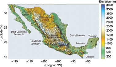
Fig. 1 Elevation map of Mexico including its main topography features. The most representative climate regions are indicated. The points represent the position of the considered stations. 

For this research work, we consider monthly means of temperature maxima (January = T1 to December = T12), monthly means of temperature minima (January = t1 to December = t12) and monthly means of accumulated precipitation (P) (36 variables in total), for a period from 1961 to 2004. In order to obtain a matrix of average values, we included stations with continuous information during the considered period and those with no more than 2% missing data. Precipitation and temperature values were evaluated using quality controls similar to ^{Zhu and Lettenmaier (2007}). The variables were standardized to a 0 mean and a standard deviation of 1. No methods were applied to fill missing data.

2.2 Principal components

The PCA was implemented as described in ^{Gong and Richman (1995}). The data matrix was used to compute the covariance between all variables or entities (A). The data matrix X contains n stations and m variables (2324 × 36). The n × m data matrix yielded a m × m matrix. Since data were standardized the resulting product matrix of the anomalies would be a standardized anomaly matrix, also known as a correlation matrix. As mentioned by ^{Estrada et al. (2009}), a correlation matrix is used to avoid that variables with larger magnitudes would dominate in the PCA results. The matrix was diagonalized into a m × m matrix of eigenvalues and a matrix of eigenvectors. The eigenvectors were scaled by the square root of the corresponding eigenvalue. Once this was accomplished, some assessment of dimensionality is often applied to reduce the m new variables (the principal components) to a smaller set, r (^{Gong and Richman, 1995}). For this research, we retained the principal component with eigenvalue > 1.

The m × r matrix was transformed by a varimax orthogonal rotation to obtain an m × r matrix of rotated principal component loadings. From these rotated loadings, an n × r set of principal component scores are formed and a Euclidian distance measure is applied to those scores. The distances are used as inputs for the cluster analysis.

This PCA has the goal of replacing the correlated climatic original variables with new components, which are mutually uncorrelated based on the principle that each component is defined by an orthogonal basis (^{Richman, 1981}). Thus, the eigenvector matrix resulting from this type of PCA is often truncated. retaining PC with eigenvalues ≥ 1 (^{Gong and Richman, 1995}).

The entries of this matrix, the eigenvectors or loadings, define new variables, consisting of linear transformations of the original variables. Thus, PCA generates another matrix that represents new uncorrelated variables (^{Richman, 1981}).

2.3 Cluster analysis

Hierarchical cluster analysis (HCA) allocates a set of objects into groups or clusters on the basis of some measurement of similarity. This similarity or distance is an Euclidean measurement, i.e., it is a simple difference between two objects (^{Fovell and Fovell, 1993}; ^{Karlsen and Elvebakk, 2003}).

Agglomerative cluster is an algorithm that starts with n clusters, each containing one single object, and then neighbor cluster pairs merge iteratively at each step to create new clusters (^{Elmore and Richman, 2001}). Thus, the number of remaining clusters is reduced by one after every step and the procedure finishes when only one cluster containing all the objects is created (^{Karlsen and Elvebakk, 2003}).

In order to identify the minimum number of suitable clusters, a K-means clustering was carried out to group the data based on similarity of PC’s. The K-means algorithm is a convergent method where k seed points are specified as a set of centroids of k clusters. The Euclidean distance is computed; then each entity is assigned to a cluster having the nearest centroid to attain an initial partition. The minimum cluster number is determined under a convergent criterion by comparing the distances to all the k clusters centroids.

Once a maximum number of clusters were obtained, we carried out an agglomerative hierarchical clustering using Ward’s method, which is an agglomerative hierarchical cluster method that merges cluster pairs with the smallest inter-cluster Euclidean distance. Ward’s method, the most frequently used for climatic classification (^{Kalkstein et al., 1987}), utilizes inter-cluster minimum variance as the distance criterion for merging cluster pairs that show the minimum squared distance between centroids (^{Fovell and Fovell, 1993}; ^{De Gaetano, 1996}). Ward’s algorithm was carried out for the retained components from the PCA to obtain a climatic regionalization (^{Kalkstein et al., 1987}). Since our final goal is the delimitation of climatic regions, every cluster will be classified using the Köppen climate classification modified by ^{García (2004}).

2.4 Silhouette coefficient

In order to determine the minimum cluster, the silhouette coefficient (SC) was computed. The method of silhouette coefficients combines both cohesion and separation (^{Tan et al., 2005}).

In order to compute the silhouette coefficient for an individual point, a process that consists of the following three steps is carried out: 1) for the ith object, its average distance to all other objects in its cluster ai’ is calculated; 2) for the ith object and any cluster not containing the object, the average distance to all the objects in the given cluster is calculated; the minimum value with respect to all clusters is bi; and 3) for the ith object, the silhouette coefficient is Si = (bi - Ui)/max(ai’ bi)’.

The value of the silhouette coefficient can vary between -1 and 1. A negative value is undesirable because it corresponds to a case in which Ui, the average distance to points in the cluster, is greater than bi, the minimum average distance to points in another cluster. We want the silhouette coefficient to be positive (ai < bi), and for ai to be as close to 0 as possible, since the coefficient assumes its maximum value of 1 when Ui = 0. We can compute the average silhouette coefficient of a cluster by simply taking the average of the silhouette coefficients of points belonging to the cluster.

3.1 Principal component analysis

Figure 2 shows PC loadings for the three first components; it is possible to observe that all variables are grouped on different sectors. PCA results show a distribution of temperatures associated to the first principal component (PC1) and precipitation variables associated to the second component (PC2). PC loadings are characterized by temperature variables through the PC1 with an explained variance of 52.9% and by precipitation variables through the PC2 with an explained variance of 19.2%. The first three principal components amounted to 82.1% of the total explained variance. Additional components had a lower effect on variance explanation (eigenvalue < 1).

Fig. 2 Plot of principal components scores PC1, PC2, and PC3 for the 1961-2004 dataset. Precipitation (P) variables are represented in PC2 while PC1 is totally explained by maximum (T) and minimum (t) temperatures, respectively. PC3 represents seasonal variability. 

As shown in Figure 2, monthly means of minimum temperature had the highest contribution to PC1, revealing the large variability of this parameter. For instance, from an average temperature of 24 ºC in warmer climates (state of Tabasco) to -4.25 ºC in colder ones (in the western Sierra Madre of Chihuahua, see Fig. 1). It is reflected in major correlation values for these variables (from November to March). Maximum temperatures are associated with negative loadings in PC2 except from January to March. Less variability in temperature is observed through all data for spring and summer months. In contrast, PC3 shows an influence of summer temperatures and for precipitation in winter months.

3.2 Cluster analysis

In order to generate the climate classification, it is necessary to delineate groups of stations which share similar meteorological characteristics. This delimitation was carried out by applying Ward’s agglomerative hierarchical clustering to the three first retained principal components. The spatial interpolation was done using a geostatistical ordinary kriging method and an exponential variogram in order to represent each cluster in its geographical context. Krigging was used to interpolate the position of the stations in the climatic groups. We used the cluster number assigned to each station after clustering. Once the interpolation was carried out, the climatic classification was performed for each cluster. Based on the results of the SC we examined the 12-level clustering solution (Table I).

Table I Characteristics of the clusters produced by clustering analysis. 

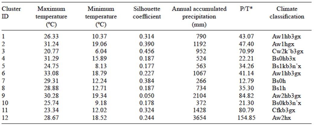
* P/T = mean annual precipitation/mean annual temperature.

The average silhouette coefficient is always positive for all clusters, though some values are relatively low (close to 0) for specific groups of stations that present exceptional rainy climates (cluster 9). For these stations, grouped into clusters with larger SC values, the ranges of precipitation and temperature are low.

3.3 Climate regions classification

Clusters 4 and 5 reflect the semiarid climate regions (BSh and BSk) from the central part of Mexico northwards (Chihuahuan Desert). These climates present low seasonal precipitation during summer due to a subtropical high-pressure zone and as a result of the geographical barriers of the main mountain ranges of Mexico. The difference between these two climates is the maximum temperature for the warm months (from May to July). Other arid zones that include the Sonoran Desert and the Baja California Peninsula were grouped in clusters 7 and 8 (BS0 and BS1). Despite their statistical similitude in terms of temperature values, cluster 7 clearly defined areas within the region delimited by cluster 8 with a difference in total precipitation and low precipitation/temperature (P/T) ratio.

The transition between the southernmost part of the highlands (2000 masl) and the area in which the western and eastern Sierra Madre converge in the central highland are defined in clusters 1, 2 and 9. Cluster 9 (AW2) delimited the transition between temperate and humid climates near the Western Sierra Madre. The wetter climate regions in the southeastern part of Mexico were grouped in clusters 3 and 11 (Cwmh and Cfh) defining the humid and temperate climate regions. These regions are located in the coastal plains, in the Yucatán Peninsula and in the highlands of Chiapas. Cluster 11 (Cfh) delineated all of the central mountain formations from the western Sierra Madre to the lowlands (El Bajío) in the central part of Mexico. Overall, the Yucatán Peninsula and regions in the coastal zone of the Gulf of Mexico are contained in cluster 2 (Aw1), which thus defined the rainy climates. Cluster 1 (AW1b3) is located in the regions of tropical rainy forests with a seasonal precipitation regime and temperate climate. The rainiest climate regions are delimited by clusters 11 (Cfk) in Tabasco and the southeast of Chiapas, where usually tropical cyclones impact (^{García, 2004}).

The P/T relation gives us an idea of the similitude between stations or groups. For instance, clusters 9 and 12 represent the same climate classification but under a different P/T regime. Thus, while cluster 9 has a P/T ratio of 84.82, for cluster 10 the ratio is 154.85. This means that large precipitations are most influenced by events such as tropical cyclones.

There are some implications for climate regionalization under global climate changes. Obviously, the present climates distribution will suffer changes for specific variables. In arid and semiarid regions in Mexico, the diurnal temperature oscillation has changed, mainly in its lower limits (^{Brito-Castillo et al., 2010}). There is also a negative trend in soil moisture content from mid-latitude zones to the north-central region of Mexico, mainly due to low precipitation. This indicates a negative change in effective daily precipitation above 1 mm (^{Seager et al., 2007}). These features needs to be considered in futures works on regional and local climate research.

3.4 Vegetation and climatic regions

Climate and topography control the distribution of many plants (^{Kelly and Goulden, 2008}). Different species of plants have suffered some effects due to changes in temperature, especially during daytime. This has caused a variation in the species composition in latitudinal and altitudinal gradients (^{Chen et al., 2011}). Another important factor is the variation of drought periods that can affect the composition of species through the seed establishment of new individuals. In addition, areas of native vegetation have been modified and disturbed by the direct action of human activities. The intensification of these activities has impacted simultaneously with the changing climate conditions at a regional scale. In many cases, the vegetation groups include, at least partially, communities that cannot be categorized as climax, but its existence is largely linked to the characteristics of the substrate (^{Miranda and Xolocotzi, 1963}; ^{Chapin et al., 2011}). The present knowledge about land vegetation cover in Mexico does not allow comparative assessments in sufficient detail, except for specific sites and at a small scale (^{Rzedowski, 2006}). Studies on vegetation are mainly focused on major vegetation types and they only show vegetation types as the basic unit of work. From the dynamic point of view, all vegetation types are described as stable biotic communities or plants based on the factors of the physical environment in which they live. For instance, although there are forests classified as secondary (mainly pine), others are the original plant or a mixture of both. Thus, vegetation types are grouped by dominant vegetation type in representative groups (^{Miranda and Xolocotzi, 1963}). However, in this research work, we can infer reconstructions of the original vegetation. It is also possible to observe a relationship between the recent dominant vegetation and climate classification. This can be seen in Figure 3.

Fig. 3 Partial distributions of vegetation groups for climate type classification. 

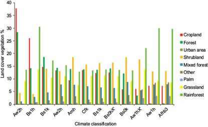
Figure 4a shows the climate regionalization by using the Ward algorithms of HCA outputs. In Figure 4b the climatology of ^{García (2004}) is included. In the climate maps of García, more detail is included regarding the types and subtypes of climates. In the climate regionalization of this study only the main climatic types of Mexico are considered, as it is observed in Figure 4c. The foremost similarities are shown for the main zones of the principal climatic groups, Aw1, Aw2, B1, B0, Cf and C. These are generally distributed in the same regions as those proposed by ^{García (2004)}. The main differences are observed in the boundaries of each type of climate, since the allocation of climate regionalization is based on totally different methodologies and philosophies. While ^{García (2004)} includes geographic and topographic assessment criteria for boundary assignment, we base spatial boundary assignments on geostatistical techniques.

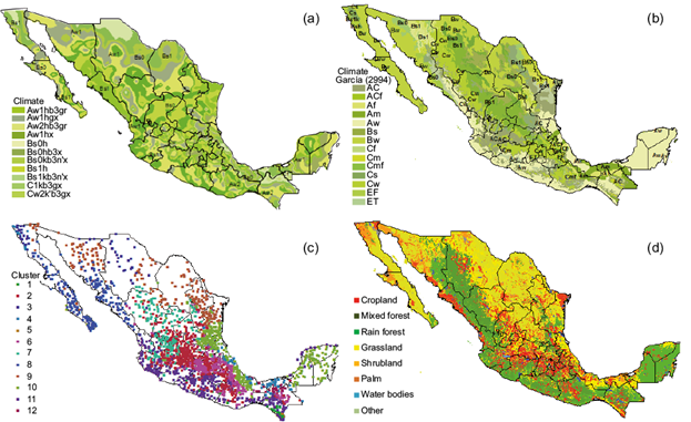
Fig. 4 (a) Climate regionalization types correspond to clustered regions; (b) Climate classification of Köppen modified by ^{García (2004}); (c) Stations grouped by cluster number; (d) Major vegetation groups in Mexico. 

Figure 4d shows the cover vegetation; it is observed a pattern width of dominant crops in climates Bs and Aw, principally where rain-fed crops are established. Historically crops were established in rangelands of dominant grasslands landscapes.

Arid and semi-arid climates (type) B cover most of the Mexican territory from the northwest in the peninsula of Baja California, and especially in the central-north region. This region is defined by a geographic effect. The differences in altitude between the center highlands and the coastal plains result in a large climate mosaic and vegetation gradient. Furthermore, the arrangement of mountains directly influences the distribution of moisture and temperature ranges. These factors partially define the aridity of that region known as the Altiplano. The large proportion of continental land in the north part of Mexico is characterized by arid regions that limit areas of scrubland and grassland. Therefore, grasslands are widely distributed in these climatic regions, with precipitation conditions as the main driver, expressed in different representative species of grassland within each region. For example, semiarid grasslands of the Chihuahuan Desert can be distinguished in the semi-dry and cold climate BS0 and Bs1 groups.

The northwestern part of Mexico is significantly affected by a high-pressure cell for most of the year increasing the degree of aridity (^{Mosiño and García, 1973}). Additionally, this region is directly influenced by a cold Pacific Ocean current that has a noticeable effect on the climate of the Baja California peninsula and of the state of Sonora, which drives the vegetation of this region, marked by the dominance of arid spiny shrubland distinctive of Bs0 climates. Shrublands are almost uniformly distributed throughout almost all of the climatic regions due to the large number of species and groups of shrubs found in Mexico. Nevertheless, it is possible to make a sub-classification of types of shrubland in correlation with the climatic classification in a gradient of moisture, from semi-desert scrubs in regions with annual average rainfall of 300 mm, to xeric scrub in regions with precipitation of 500-650 mm.