1. Introduction

The changes in climate experienced during the recent decades already had widespread impacts on human and natural systems (^{IPCC, 2014a}). The description of trends in temperature series and their attribution to anthropogenic and natural factors is central to understanding the response of the climate system to changes in external forcing, the role of human activities in altering this system, and how the risk of larger impacts might be mitigated. As has been widely discussed in both the academic and political arenas, the implications of further significant anthropogenic warming are far reaching and may call for considerable changes in economic, technological and societal trends (^{Stern, 2007}; ^{IPCC, 2014b}; ^{van den Bergh and Botzen, 2014}).

Despite the differences in approaches (physical- or empirical-based), the existence of strong methodological debates (^{Triacca, 2005}; ^{Estrada et al., 2010}; ^{Estrada and Perron, 2014}), as well as important mismatches between climate models’ reconstructions and observations (^{Stocker et al., 2013}; ^{Fyfe et al., 2016}), almost all of the attribution studies to date arrive to the same conclusion: observed warming is anywhere from partially to dominantly anthropogenic (^{Bindoff et al., 2013}). However, even if the attribution of the observed warming to human activities is no longer in question, there is still a need to improve and develop methods that can help to better understand how this phenomenon has manifested itself and to better gauge human interventions in the different expressions of a warming climate. In particular, it is important to extend current methodologies for detecting and attributing changes in the rate of warming, such as periods of fast warming, slowdowns and pauses. These are currently the most relevant policy and scientific aspects in the fields of detection and attribution of climate change (^{Tollefson, 2014}; ^{Estrada and Perron, 2016}; ^{Tollefson, 2016}; ^{Kim et al., 2017}). For this matter, it is important to distinguish between the observed temperature trends and the underlying warming trends. The first is affected by natural variability, especially low-frequency oscillations, that can have similar magnitudes than the response produced by changes in external forcing factors and can significantly modify the underlying warming trends (^{Dima et al., 2007}; ^{Swanson et al., 2009}; ^{Semenov et al., 2010}; ^{Wu et al., 2011}; ^{Estrada et al., 2013a}, ^b; ^{Steinman et al., 2015}). The second is harder to obtain as it implies not only being able to attribute climate change to its different natural and anthropogenic causes but also to successfully extract the warming trend from the effects of these large natural variations. Extracting this trend is required to investigate the effects of changes in anthropogenic forcing on the warming rates of the climate system. The apparent slowdown in the warming provides a good example about the need of distinguishing between observed temperature series and the underlying warming trend. Year 2015 was the warmest on record by a considerable margin, does this imply that the slowdown in the warming has ended? Does it imply that the slowdown never really existed? Recent papers have analyzed unfiltered global temperature series and have concluded that the recent slowdown was either an artefact of the data or that it never really happened (^{Foster and Rahmstorf, 2011}; ^{Karl et al., 2015}; ^{Cahill et al., 2015}; ^{Lewandowsky et al., 2015}, ²⁰¹⁶). A large part of the body of research on this topic has concluded that the apparent hiatus could be produced by the effects of low-frequency natural variability represented by physical modes such as AMO, NAO and PDO (^{Li et al., 2013}; ^{Trenberth and Fasullo, 2013}; ^{Steinman et al., 2015}; ^{Guan et al., 2015}). These modes can mask the warming trend and create the illusion of a slowdown in the underlying warming trend. However, it is important to realize that these questions refer to the underlying warming trend and cannot be properly answered if the effects of natural variability - particularly low-frequency oscillations, but also shorter-term variations such as El Nino/Southern Oscillation (ENSO) - are not taken into account.

^{Estrada and Perron (2016}) proposed a method based on cotrending testing and the application of a Principal Component Analysis (PCA) to extract the underlying common trend in global and hemispheric temperatures. They showed that some modes of natural variability could considerably distort the underlying warming trend, making difficult to investigate the existence of the current slowdown of the warming unless the underlying trend is purged from the effects of natural variability. Their results show that the slowdown cannot be explained away by natural variability and that it is a statistically significant feature of the underlying warming trend. Recently, a new approach for testing for the attribution of changes in the rate of warming was developed by ^{Kim et al. (2017}). It is based on new structural change tests that allow making inference about common breaks in a multivariate system with joined segmented trends. They concluded that the breaks in radiative forcing as well as in global and hemispheric temperatures are common and that since the 1990s there has been a significant decrease in the rate of growth of both temperatures and radiative forcing. ^{Estrada and Perron (2016)} and ^{Kim et al. (2017)} show that the existence of the slowdown in the warming can be properly tested if the effects of natural variability are filtered out and if adequate statistical tests are used for this task. Their results provide strong evidence for the existence of the current slowdown and for its dominant anthropogenic origin as was previously suggested (^{Estrada et al., 2013b}).

In this paper, we characterize both the observed and underlying warming trends in hemispheric sea and land surface temperatures. We document important differences in the observed nonlinear trends in these temperature series, which would suggest that the northern and southern hemispheres have responded very differently to the observed changes in the radiative forcing. However, once the observed temperatures are purged from natural variability, it is shown that these series share the same underlying warming trend. Furthermore, the time-series analysis of the interhemispheric temperature asymmetry (ITA) suggests that the differences in warming between hemispheres are mainly due to natural variability, and not so much to differences in the response to increases in radiative forcing.

The rest of this paper is structured as follows. Section 2 describes the data and the univariate and multivariate methods used. The time series properties and the analysis of the trends in land and sea temperature series are presented and discussed in Section 3. The existence of a common secular trend between sea and land temperatures and radiative forcing is investigated in Section 4. These results are used to study the attribution of the trend in ITA and its features. Section 5 is concerned with the extraction and description of the common trend in radiative forcing and hemispheric land and sea temperatures. Section 6 concludes and summarizes the main findings.

2. Data and methods

The land and sea surface temperature series (Fig. 1) were obtained from the Climatic Research Unit (CRU; ^{Morice et al., 2012}) and NASA (^{Hansen et al., 2010}). Note that the NASA dataset contains only global but not hemispheric sea surface temperature series. For the rest of the paper, sea, land, and sea and land temperatures are denoted by the letters S, L and SL, and the accompanying superscript identifies the dataset (H for CRU, and N for NASA) and region (G, NH and SH for global, northern hemisphere and southern hemisphere, respectively). The following indices are used to represent inter-annual variability (Fig. 2): the Atlantic Multidecadal Oscillation (AMO; ^{Enfield et al., 2001}); the Southern Oscillation Index (SOI; ^{Trenberth, 1984}), the North Atlantic Oscillation (NAO; ^{Hurrell, 1995}) and the Pacific Multidecadal Oscillation (PDO; ^{Zhang et al., 1997}). The radiative forcing data (in W/m²) was obtained from NASA (Hansen et al., 2011). For the analyses presented in this paper, we use (Fig. 3): 1) the well mixed greenhouse gases (WMGHG; carbon dioxide (CO₂), methane (NH₄), nitrous oxide (N₂O) and chlorofluorocarbons (CFCs)); 2) the total radiative forcing (TRF) which includes WMGHG plus ozone (O₃), stratospheric water vapor (H₂O), solar irradiance, land use change, snow albedo, black carbon, reflective tropospheric aerosols and the indirect effect of aerosols, and; 3) the radiative forcing from stratospheric aerosols (STRAT).¹ The data are annual and the samples available are: 1850-2015 for Hadley temperatures (with the exception of G and SH land temperatures which start in 1856); 1880-2105 for NASA temperatures; 1880-2011 for the radiative forcing; 1856-2015 for AMO; 1866-2014 for SOI, 1850-2015 for NAO; 1854-2015 for PDO.

Fig. 1 Global and hemispheric temperature series from CRU and NASA datasets. (a) SL from the CRU dataset (H) for global (SLH_G), northern hemisphere (SLH_NH) and southern hemisphere (SLH_SH); (b) SL from the NASA dataset (N) for global (SLN_G), northern hemisphere (SLN_NH) and southern hemisphere (SLN_SH); (c) L from H for global (LH_G), northern hemisphere (LH_NH) and southern hemisphere (LH_SH); (d) L from N for global (LN_G), northern hemisphere (LN_NH) and southern hemisphere (LN_SH); (e) L from H for global (SH_G), northern hemisphere (SH_NH) and southern hemisphere (SH_SH); (f) S from N for global (SN_G). 

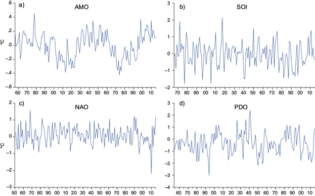
Fig. 2 Principal modes of natural variability. (a) Atlantic Multidecadal Oscillation (AMO). (b) Southern Oscillation index (SOI); (c) North Atlantic Oscillation (NAO); (d) Pacific Decadal Oscillation (PDO). 

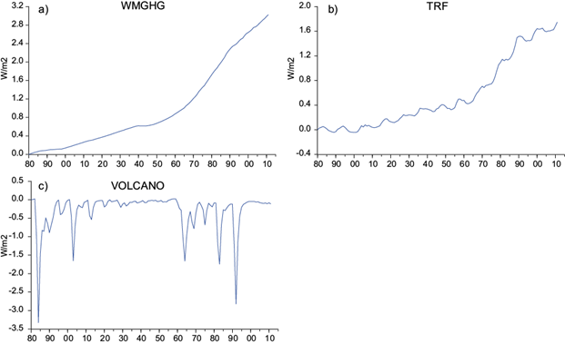
Fig. 3 Radiative forcing series. (a) Well-Mixed Greenhouse Gases (WMGHG); (b) Total Radiative Forcing (TRF); (c) radiative forcing from stratospheric aerosols (STRAT). 

We next briefly describe the methods used in the empirical applications. Our descriptions are brief and simply present the main ideas. The reader is referred to ^{Estrada and Perron (2014)} for more details.

2.1 Perron-Yabu testing procedure for structural changes in the trend function

^{Perron (1989)} showed that the presence of structural changes in the trend can have considerable implications when investigating time-series properties by means of unit root tests. This creates a circular problem given that most of the tests for structural breaks require to correctly identify if the data generating process is stationary or integrated. Depending on whether the process is stationary or integrated the limit distribution of these tests are different and, if the process is misidentified, the tests will have poor properties. Building on the work of ^{Perron and Yabu (2009a)}, the Perron and Yabu ^{(PY; 2009b)} test was designed explicitly to address the problem of testing for structural changes in the trend function of a univariate time series without any prior knowledge as to whether the noise component is stationary, I(0), or contains an autoregressive unit root, I(1).

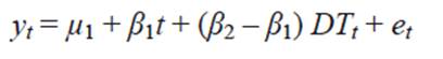
We present the case of a model with a one-time structural break in the slope of the trend function with an autoregressive noise component of order one (AR(1)); the case with general types of serial correlation in the noise is somewhat more involved (see ^{Perron and Yabu, 2009}b, for details), though the main ingredients are similar. Consider the following data generating process:

(1)

where e _t ~ i.i.d. (0, σ ²) and DT _t = (t - T _B ) if t > T _B and 0 otherwise so that the trend function is joined at the time of the break. The autoregressive coefficient is such that -1 < α ≤ 1 and therefore, both integrated and stationary errors are allowed. The break date is denoted T _B = [λT] for some λ ∈ (0,1), where [·] denotes the largest integer that is less than or equal to the argument and 1(·) is the indicator function. The hypothesis of interest is β ₁ = 0.

The testing procedure is based on a Quasi Feasible Generalized Least Squares approach that uses a superefficient estimate of α when α = 1. The estimate of α is the OLS estimate obtained from an autoregression applied to detrended data and is truncated to take a value 1 when the estimate is in a T ^-δ neighborhood of 1. This makes the estimate “super-efficient” when α = 1. Theoretical arguments and simulation evidence show that δ = 1/2 is the appropriate choice. Treating the break date as unknown, the limit distribution is nearly the same in the I(0) and I(1) cases when considering the Exp functional of the Wald test across all permissible dates for a specified equation, see ^{Andrews and Ploberger (1994}). To improve the finite sample properties of the test, they also use a bias-corrected version of the OLS estimate of α as suggested by ^{Roy and Fuller (2001}). The testing procedure suggested is: (1) For any given break date, detrend the data by Ordinary Least Squares (OLS) to obtain the residuals ; (2) estimate an AR(1) model for yielding the estimate ; (3) use to get the Roy and Fuller (2001) biased corrected estimate M; (4) apply the truncation MS = M if |M - 1| > T-1/2 and 1 otherwise; (5) apply a Generalized Least Squares (GLS) procedure with _MS to obtain the estimates of the coefficients of the trend and the variance of the residuals and construct the standard Wald-statistic W _FMS (λ) to test for a break at date T _B = [λT]; (6) repeat the five steps above for all permissible break dates to construct the Exp functional of the Wald test denoted by Exp - WFS = log[T ^-1 ∑_Λ exp (W _FMS (λ) /2)] where Λ = {λ; ε ≤ λ ≤ 1 - ε} for some ε > 0. We set ε = 0.15 as is common in literature.

2.2 Perron and Kim-Perron unit root tests with a one-time break in the trend function

^{Perron (1989}) proposed an extension of the Augmented ^{Dickey-Fuller (ADF) test (Dickey and Fuller, 1979}; ^{Said and Dickey, 1984}) that allows for a one-time break in the trend function of a univariate time series. Our interest centers on the “changing growth” model, which can be briefly described as follows. The null hypothesis is:

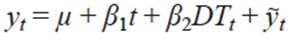
where DU _t = 1 if t > T _B , 0 otherwise; T _B refers to the time of the break, and e _t is some stationary process. The alternative hypothesis is:

where DT _t = t - T _B ; if t > T _B and 0 otherwise. The “changing growth” model takes an “additive outlier” approach in which the change is assumed to occur rapidly and the regression strategy consists in first detrending the series according the following regression:

(2)

A problem with most procedures to test for a unit root in the presence of a one-time break that occurs at an unknown date (e.g., Zivot and Andrews [1992] and some of the tests in ^{Perron [1997}]) is that the change in the trend function is allowed only under the alternative hypothesis of a stationary noise component. As a consequence, it is possible that a rejection occurs when the noise is I(1) and there is a large change in the slope of the trend function. A method that avoids this problem is that of ^{Kim and Perron (2009}). Their procedure is based on a pre-test for a change in the trend function, namely the PY test. If this pre-test rejects, the limit distribution of their modified unit root test is then the same as if the break date was known (^{Perron and Vogelsang, 1993}). This is very advantageous since when a break is present the test has much greater power. The testing procedure for the changing growth model consists in the following steps: (1) Obtain an estimate of the break date by minimizing the sum of squared residuals using regression (2); then construct a window around that estimate defined by a lower bound T _l and an upper bound T _h . A window of 10 observations was used. Note that, as shown by ^{Kim and Perron (2009)}, the results are not sensitive to this choice. (2) Create a new data set {y ⁿ } by removing the data from to T _l + 1 to T _h , and shifting down the data after the window by S(T) = ; hence,

(3) Perform the unit root test using the break date T _l . This is the t-test statistic for testing that = 1 in the following regression estimated by OLS, denoted by :

(3)

where = T _l /T _r , T _r = T - (T _h - Tl) and is the detrended value of y ⁿ .

2.3 Perron-Zhu methodology for constructing a confidence interval for the break date

^{Perron and Zhu (2005}) analyzed the consistency, rate of convergence and limiting distributions of parameter estimates in models where the trend exhibits a slope change at some unknown date and the noise component can be either stationary or have an autoregressive unit root. Another important practical application of deriving the limiting distribution of the estimate of the break date is that it permits forming a confidence interval for the break date. Of the various models considered in that paper, the joint-segmented trend model with stationary errors is the most relevant to our applications (e.g., ^{Gay et al., 2009}; ^{Estrada et al., 2013}a,b), in which case the regression of interest is

estimated by OLS. Denote the resulting estimate by and the associated estimate of the break fraction by = /T. They showed that the limit distribution of the break fraction is:

where is thetruevalue of thechangein the slopeparameter and σ ² is the long-run variance of u _t estimated using the Bartlett kernel with ^{Andrews’ (1991}) automatic bandwidth selection method using an AR(1) approximation.

2.4 Bierens’ nonparametric nonlinear co-trending test

The advantage of the co-trending test proposed by ^{Bierens (2000}) is that the nonlinear trend does not have to be parameterized. The nonlinear trend stationarity model considered can be expressed as follows:

with

where z _t is a k-variate time series, u _t is a k-variate zero-mean stationary process and f (t) is a deterministic k-variate general nonlinear trend function that allows, in particular, structural changes. Nonlinear co-trending occurs when there exists a non-zero vector θ such that θ' (t) = 0. Hence, the null hypothesis of this test is that the multivariate time series z _t is nonlinear co-trending, implying that there is one or more linear combinations of the time series that are stationary around a constant or a linear trend.

The nonparametric test for nonlinear co-trending is based on the generalized eigenvalues of the matrices M _l and M ₂ defined by:

where if with and being the estimates of the vectors of intercepts and slope parameters in a regression of z _t on a constant and a time trend; also

where m = T ^α with T the number of observations and α = 0.5 as suggested by ^{Bierens (2000}). Solving and denoting the r-th largest eigenvalue by , the test statistic is . The null hypothesis is that there are r co-trending vectors against the alternative of r - 1 co-trending vectors. This test has a non-standard distribution and the critical values have been tabulated by ^{Bierens (2000)}. The existence of r co-trending vectors in r + 1 series indicates the presence of r linear combinations of the series that are stationary around a linear trend and that these series share a single common nonlinear deterministic trend. Such a result indicates a strong secular co-movement in the r + 1 series.

3. Time-series properties and trends in observed land and sea surface temperatures and radiative forcing

Temperature series have been typically represented either as trend-stationary or difference-stationary processes (^{Tol and de Vos, 1993}; ^{Kaufmann and Stern, 1997}; ^{Gay-García et al., 2009}). Determining which process better represents these series generated a long debate in the literature (for a review see ^{Estrada and Perron, 2014}). Besides the theoretical implications that these differences can have, describing temperatures and radiative forcing as difference-stationary or trend-stationary processes could have important practical implications for observation-based attribution studies. However, the vast literature has also shown that the attribution of climate change to human intervention with the climate system is robust to assuming temperature and radiative forcing variables as being all trend-stationary or all first difference-stationary (^{Tol and de Vos, 1998}; ^{Stern and Kaufmann, 1999}; ^{Estrada et al., 2013b}; ^{Estrada and Perron, 2016}).

In this section, we analyze by means of state-of-the-art econometric techniques the time-series properties of hemispheric land and sea temperatures and radiative forcing. The most common tools for investigating the data generating process of temperature series are unit root tests (^{Estrada and Perron, 2014}). However, the results of these tests are highly sensitive to the presence of structural changes in the trend function (^{Perron, 1989}): if there is a shift in the trend function the sum of the autoregressive coefficients is highly biased toward unity and therefore the unit root null is hardly rejected even if the series are composed of white noise realizations around the trend; moreover, if the break occurs in the slope of the trend, the null of a unit root cannot be rejected even asymptotically.

The rate of warming during the observed period has not been constant and the existence of changes in the slope of the trend functions of climate variables is not only expected, it has also been widely reported (^{Seidel and Lanzante, 2004}; ^{Tomé and Miranda, 2004}; ^{Estrada et al., 2013b}; ^{Estrada and Perron, 2016}). As such, the first step is to investigate the existence of breaks in the trend function by means of a testing procedure that is robust to whether temperature variables are difference- or trend-stationary. Then, the nature of the data generating process for these series can be investigated. The PY test provides a robust way to investigate the existence of structural breaks in the trend function without the need to know if the series is difference- or trend-stationary (Perron and Yabu, 2009). This characteristic makes this test particularly useful as a pretest for applying the adequate type of unit root tests.

Table I shows that the PY test results indicate that a break in the slope of the trend function is present in all series, with the exception of the northern hemisphere S _H . The large differences in the break date estimates for the various temperature series is notable, ranging from 1909 to 1984. Sea and southern hemisphere tend to show breaks in the slope of the trend function at the beginning of the 20th century, while for northern hemisphere and land temperature series, the break dates occur in the second part of the century. In contrast, for both TRF and WMGHG the break dates are estimated to occur at the same time during the second part of the 20th century. The rates of warming over the observed period are markedly different between hemispheres, as well as between sea and land (Tables IIa, b, c). All sea temperatures show a moderate cooling trend starting in the late 19th century and the early part of the 20th (about -0.2 ºC to -0.3 ºC per century, with the exception of S from NASA which shows a much larger trend of -0.94 ºC per century). A similar cooling trend (about -0.14 ºC per century) is found in SL temperatures over the southern hemisphere, which is dominantly composed of oceans. These trends are consistent with the effects of ocean cooling trends that have been documented from the preindustrial times until the beginning of the 20th century, when the increase in anthropogenic forcing started to become more important (^{Delworth and Knutson, 2000}; ^{Stott et al., 2000}; ^{McGregor et al., 2015}; ^{Abram et al., 2016}). For all sea temperature series, a moderate warming started after 1909 and, in the case of the southern hemisphere SL, the warming started after 1925 (in all cases the rate of warming is about 0.7 ºC per century). While the post-break differences in hemispheric warming are small regarding sea temperatures, the differences in the warming rate are very large for land temperatures. Warming trends over land in the northern hemisphere are about twice those of the southern hemisphere (about 3.2 and 1.6 ºC per century, respectively). These relative magnitudes are largely due to the differences in the distribution of land/ocean mass between hemispheres and to the large heat capacity of the oceans (^{Peixoto and Oort, 1992}).

Table I Tests for the existence of a break in the slope of temperature and radiative forcing series. 

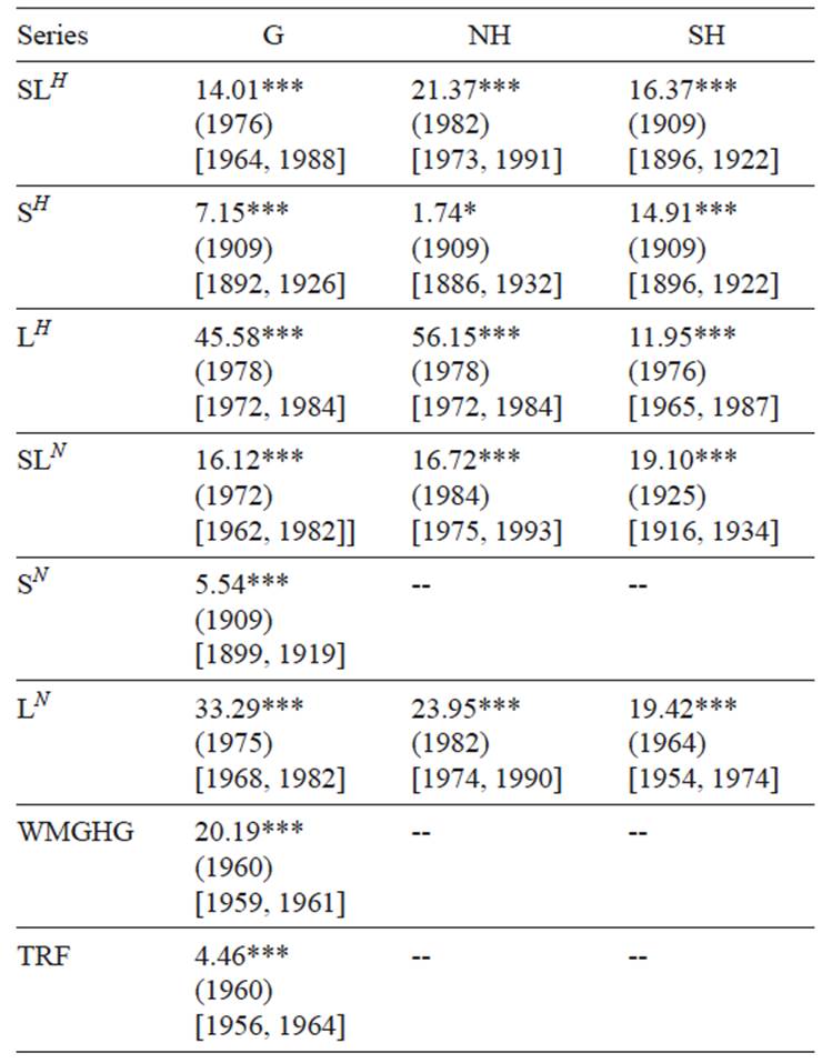
The main entries are the values of the PY test. ***,**,*, denote statistical significance at the 1, 5 and 10% levels, respectively. The estimated break dates are given in parenthesis and their corresponding 95% confidence intervals are shown in brackets.

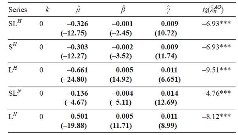
Table IIa Tests for a unit root allowing for a one-time break in the trend function applied to global temperature and radiative forcing series. 

Bold figures denote statistically significance at the 5% level. T-statistic values are given in parenthesis. tα^(λ^tr AO) is the Kim-Perron test statistic. ***,**,*, denote statistical significance at the 1, 5 and 10% levels, respectively.

Table IIb Tests for a unit root allowing for a one-time break in the trend function applied to northern hemisphere temperature series. 

Bold figures denote statistically significance at the 5% level. T-statistic values are given in parenthesis. is the Kim-Perron test statistic. ***,**,*, denote statistical significance at the 1, 5 and 10% levels, respectively.

Table IIc Tests for a unit root allowing for a one-time break in the trend function applied to southern hemisphere temperature series. 

Bold figures denote statistically significance at the 5% level. T-statistic values are given in parenthesis. is the Kim-Perron test statistic. ***,**,*, denote statistical significance at the 1, 5 and 10% levels, respectively.

If taken at face value, such large differences in warming rates and break date estimates would suggest that the existence of common secular trends and breaks between hemispheric temperatures and radiative forcing would be unlikely. Furthermore, the results would support the fact that ITA has increased during the observed period and that a larger contrast between hemispheric temperatures could be expected in the future (^{Friedman et al., 2013}; ^{Goosse, 2016}). However, as mentioned in the introduction, it is important to distinguish between observed and underlying warming trends. Low-frequency variability can lead to under- or overestimation of the warming rates and can severely affect the break date estimates (^{Swanson et al., 2009}; ^{Wu et al., 2011}; ^{Estrada et al., 2013}b; ^{Guan et al., 2015}; ^{Estrada and Perron, 2016}). To address these questions, appropriate statistical tests need to be used to investigate the time series properties of these series and the existence of a common secular trend.

The results of applying the Kim Perron test provide strong evidence in favor of trend-stationary processes with a break in the slope of their trend functions for all temperature and radiative forcing series (Tables IIa, b, c). The only exception is the northern hemisphere S ^H , for which the null hypothesis of a unit root cannot be rejected at conventional levels. These results are broadly similar with those previously reported for other temperature series (^{Gay-García et al., 2009}; ^{Estrada et al., 2013b}; ^{Estrada and Perron, 2016}). Moreover, they provide additional evidence suggesting that temperature series are better represented as trend-stationary processes, whether the measurements correspond to land or ocean and irrespective of their spatial scale (^{Gay et al., 2007}). Given that both temperature and radiative forcing series share the same type of time-series properties, the next section focusses on investigating the existence of a common secular trend by means of the co-trending test described in the methods section (^{Bierens, 2000}).

4. Testing for a common secular trend between temperatures and radiative forcing series and investigating the trend in ITA

The results in the previous section indicate strong differences in the observed characteristics of the trend functions of sea and land hemispheric temperatures, and also between radiative forcing and temperature variables. Taken at face value, the previous analysis would suggest that hemispheric sea and land temperature series follow different trends and that these are hardly related to the trends shown by radiative forcing series. Testing for cotrending provides a way to investigate the existence of an underlying common trend in temperature series and radiative forcing that might be masked by the natural variability in temperatures. Furthermore, these tests can help understanding the causes behind the underlying warming trend and to evaluate the role of human activities in warming the climate system (^{Estrada et al., 2013b}; ^{Estrada and Perron, 2014}).

In this section, the sets of variables used to apply the cotrending test are selected to address the following questions: 1) is there a common secular trend between all temperature and TRF and WMGHG?; (2) is this common trend imparted by WMGHG, which has mainly an anthropogenic origin?; (3) do global and hemispheric temperatures share the same trend across the different datasets? The first two questions are directly related to attributing the underlying warming trend to human activities and, therefore, cotrending is tested within the different temperature datasets (CRU and NASA). For the third one, the cotrending test is carried out across the different temperature datasets in order to address if the differences in how CRU and NASA process and adjust data affect the underlying trends or if these differences mainly affect the noise component of these series. As discussed below, these results are useful to investigate the systematic movement shown by ITA and its drivers.

Table III shows that for both datasets there is a common secular trend between WMGHG, TRF and all S, SL and L temperature series, at the global and hemispheric scales. These results provide strong evidence about the anthropogenic origin of the warming trend. Although statistical methods alone can hardly prove causality, the way the tests are structured and by invoking basic climate physics it is possible to establish a causal link. By construction, WMGHG is contained in TRF and therefore if these two variables cotrend, it must be that WMGHG is imparting TRF its trend; as expected form climate physics, temperatures follow the trend imparted by TRF. As such, the common trend in all series has its origins in WMGHG (^{Estrada et al., 2013}b), all other forcing factors mainly modulate this trend. Furthermore, these results confirm that the differences in the break dates reported in the previous section are due to temporary excursions from the common trend that are produced by natural variability oscillations. Section 6 provides further evidence on how natural variability modes alter the underlying common trend and its features.

Table III Cotrending tests within CRU and NASA datasets for L, SL and L, TRF and WMGHG. 

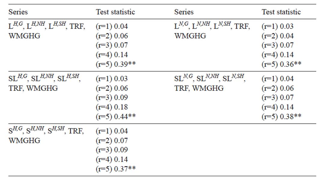
**,* denotes statistical significance at the 10 and 5% levels, respectively. r is the number of cotrending vectors. Note that S^N is only available at the global scale.

The results in Table IV complement those in Table III and strongly suggest that the differences across CRU and NASA datasets for all temperature series and scales do not affect the underlying trend: in all cases, deviations from the common trend can be considered stationary. However, as shown by the results in Table I, these deviations are large enough to severely distort the observed trend in temperatures. Note that the existence of a common trend does not preclude that significant differences in the warming rates between hemispheres could be present.

Table IV Cotrending tests across CRU and NASA datasets for L, SL and L, TRF and WMGHG. 

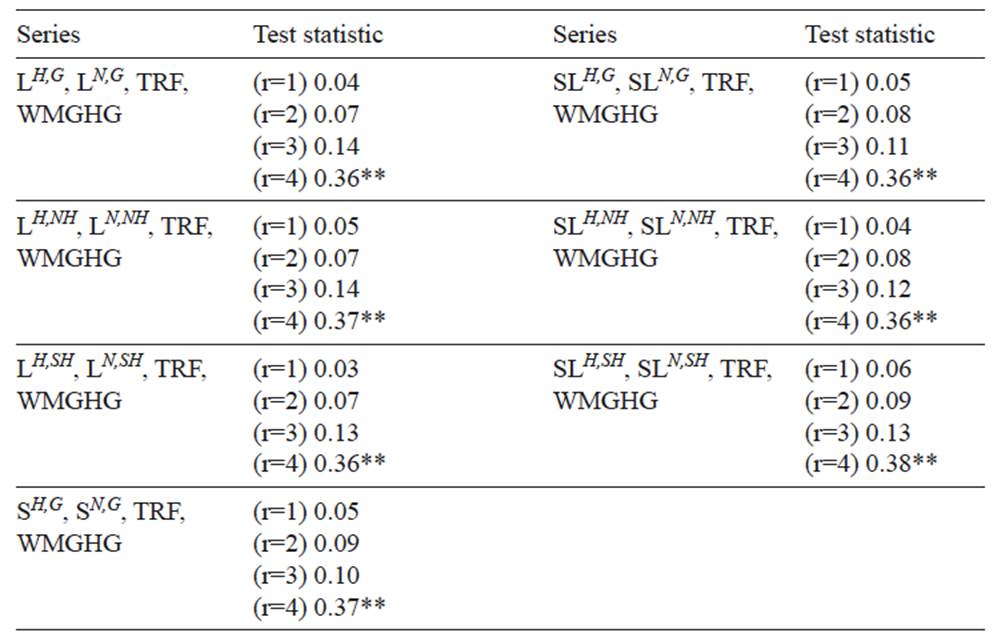
**,* denotes statistical significance at the 10 and 5% levels, respectively. r is the number of cotrending vectors. Note that S^N is only available at the global scale.

The transient climate response (TCR) relates the time-dependent change in global mean surface temperature to changes in the time-dependent change in external forcing (^{Gregory and Forster, 2008}; ^{Schwartz, 2012}; ^{Estrada et al., 2013}b). Estimates of the TCR can be obtained by regressing temperature series on TRF as follows:

(4)

Where c is a constant, γ is a fixed parameter that represents TCR and, ε _t encompasses low- to high-frequency unforced climate variability, which as indicated by the results in Tables III and IV can be assumed as stationary variations.

Table V presents the estimates of TCR and of the response of hemispheric sea/land temperatures to the observed changes in TRF. The TCR estimates obtained for global SL temperatures are broadly similar for both CRU and NASA datasets: a 1 W/m² increase in TRF would produce an increase in global temperatures of about 0.45 ºC. The difference in the response of global SL temperatures to changes in TRF between the two datasets is quite small (about 11%). The differences are also below 11% for all other global and hemispheric temperature series, with the exception of land temperature for the southern hemisphere. In that case, the response to changes in TRF for NASA is about 22% larger than that for CRU. This is probably related to how the different groups process and adjust temperature data (e.g., interpolations where data is missing).

Table V Response of temperature series to changes in TRF. 

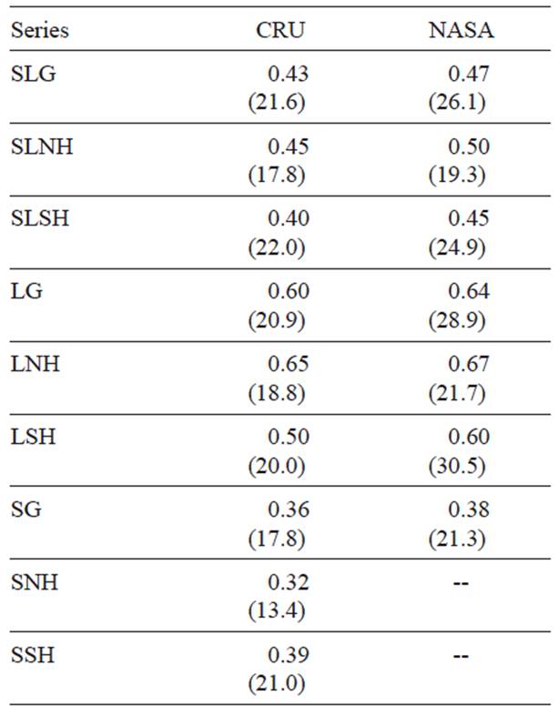
The reported values correspond to γ in (4). t-statistic values are given in parenthesis.

As expected, given the high heat capacity of the oceans, the warming induced by changes in radiative forcing is much higher over land than over sea. In particular, the largest response occurs over the northern hemisphere. This temperature difference between hemispheres is a characteristic of the Earth’s climate and has been suggested to be the result of a northward cross-equatorial ocean heat transport and the difference in the fraction of continental mass (^{Kang et al., 2015}; ^{Goosse, 2016}). The temperature contrast between hemispheres has emerged in the literature as an indicator of climate change (^{Friedman et al., 2013}). Changes in ITA linked to increases in radiative forcing are of particular interest given its potential effect in displacing the intertropical convergence zone and with it the current precipitation patterns over large parts of the world could change (^{Broecker and Putnam, 2013}; ^{Seo et al., 2016}). The observed ITA has been characterized as showing no trend during most of the 20th century but having an increasing trend of about 0.17 ºC per decade since 1980. Models simulations indicate that this temperature contrast will increase considerably in the future (^{Friedman et al., 2013}). For instance, under the RCP8.5 scenario and for the Coupled Model Intercomparison Project (CMIP5) ensemble, the projected increases in ITA for the end of this century are in the range of 0.01 to 2.96 ºC, with an ensemble mean value of 1.63 ºC. The ITA ensemble mean for the RCP8.5 scenario follows a linear trend of about 0.17 ºC per decade, which is similar to that reported for the last part of the observed period (^{Friedman et al., 2013}). However, recent studies have argued that current climate models exaggerate the synchronicity of hemispheric temperature fluctuations due to an underestimation of internal variability and feedbacks, particularly in the southern hemisphere (^{Neukom et al., 2014}). This lack of synchronicity in hemispheric natural variability could explain a large part of the observed changes in ITA. The results presented in Tables III to V allow to empirically estimate the change in ITA that can be attributed to differences in the response to external forcing from the northern and southern hemispheres. The values of γ from (4) for SL ^NH and SL ^SH show that the difference in the transient response between hemispheres is about 0.054 ºC per W/m², for both CRU and NASA. That is, if an increase in radiative forcing of 8.5 W/m² occurs by the end of this century (as is supposed under the RCP8.5 scenario), the ITA would rise only by about 0.46 ºC. This estimate is within the range of 0.01 to 2.96 ºC mentioned above, but is substantially lower than the average of the CMIP5 ensemble (1.63 ºC).²

Figure 4a shows ITA computed as the difference between SL from northern and southern hemispheres. As previously reported in the literature, visual inspection of ITA suggests the existence of a sudden drop in the late 1960s and a positive trend afterwards (^{Friedman et al., 2013}). We formally document the existence of a break in both the level and the slope of the trend function by applying the PY test to ITA. The test results show compelling evidence for such a break occurring in 1968 (PY test values of 28.04 and 17.15 for CRU and NASA, respectively). This feature persists even after the underlying warming trend is removed (i.e., after ITA is detrended using TRF; Fig. 4b).³ In this case, the PY test values are 17.67 and 14.22 for CRU and NASA, respectively. This strongly suggests that the sudden drop and positive trend shown since 1968 are the product of combining the low-frequency natural variability contained in NH and SH, which can have different amplitudes, periods and/or phases. As shown in the literature (^{Neukom et al., 2014}; ^{Abram et al., 2016}), SH and NH are characterized by differences in timing and phase of cooling and warming periods. This fact is clearly illustrated by the results in Table I. The lack of synchronicity in hemispheric natural variability could have generated the observed break in the trend function of ITA, and cause a temporary trend in the interhemispheric temperature contrast during the last decades.

Fig. 4 Interhemispheric Temperature Asymmetry. Panel a): the blue line shows ITA from the CRU dataset (ITA_H), while the red line shows ITA from the NASA dataset (ITA_N); Panel b): ITA detrended using TRF, for the CRU (ITA_H*; blue line) and NASA (ITA_N*; red line) datasets. 

To further investigate if the break in ITA can be explained by natural variability, we applied a two-step method: 1) autoregressive distributed lag models (ARDL) are estimated using TRF,AMO,NAO,SOI, and PDO as explanatory variables, which are some of the main modes of climate variability (^{Enfield et al., 2001}; ^{Trenberth, 1984}; ^{Hurrell, 1995}; ^{Zhang et al., 1997}); 2) the PY test is applied to the residuals of these ARDL regressions to test for the existence of a break in the trend function. For robustness, in this second step, the three possible types of breaks considered by ^{Perron and Yabu (2009}b) are tested for: in the level, in the slope, and in the level and slope of the trend function. The general specification of the ARDL models used is:

(5)

The number of lags for the ARDL (p, q ₁, q ₂, q ₃, q ₄, q ₅) model above is selected using the Akaike Information Criterion. The maximum number of lags in all cases was restricted to four. For the CRU and NASA datasets, the selected models were ARDL (3, 0, 1, 0, 0, 0) and ARDL (4, 0, 3, 0, 0, 0), respectively. These models explain about 53% (CRU) and 67% (NASA) of the variance of ITA, and standard misspecification tests (not shown) indicate a well-specified regression.

More importantly, Table VI shows that no break in the trend function (slope, level or both) is present after the effects of natural variability have been taken into account. These results suggest that, while anthropogenic forcing has contributed to the trend in ITA, the rapid increase shown by this variable since the late 20th century can be explained by natural variability.

Table VI Tests for the existence of a break in the level and slope, the slope and, the level of the ARDL regression residuals. 

The main entries are the values of the Perron-Yabu test. ***,**,*, denote statistical significance at the 1, 5 and 10% levels, respectively. The estimated break dates are given in parenthesis.

5. Extracting the common warming trend and investigating its features

The results in Sections 3 and 4 suggest that natural climate variability can significantly distort the underlying common warming trend in a way that the observed temperature trends seem to bear little resemblance to each other and to those of the radiative forcing series. Here we follow the approach proposed by ^{Estrada and Perron (2016}) to extract and characterize the common trend in temperature and radiative forcing series via a PCA, documented in the previous section.

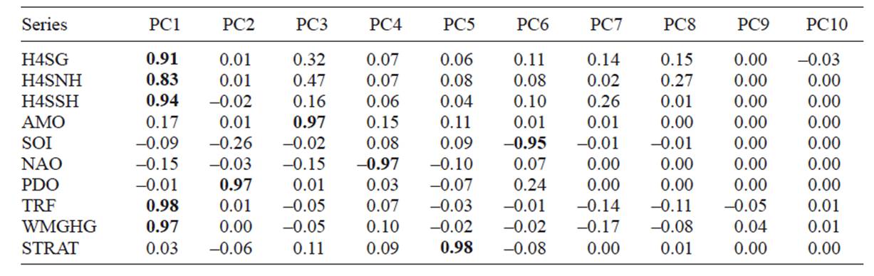
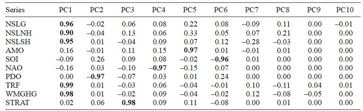
The PCA analysis to extract the common trend is carried out using sets of variables that include those used for the cotrending test in the previous section (G, NH, SH, WMGHG and TRF), the main natural variability modes (AMO, SOI, NAO and PDO), and STRAT. The analysis is done for each temperature dataset (CRU, NASA) and for SL, L and S. The PCA analysis presented here extracts and rotates the ten possible principal components for each set of variables. Note that the application of the PCA proposed in ^{Estrada and Perron (2016}) is not to reduce dimensionality but to extract the common trend from the other modes of variability. Tables VIIa, b and c show the factor loadings of the rotated PCA for the CRU dataset and Tables VIId and VIIe show those for NASA’s. In all cases, the main mode of variability is the common underlying trend represented by PC1, which is highly correlated with the radiative forcing and temperature series and has almost zero correlation with all the other variables. PC1 explains about 48% of the variability of the different sets of variables (Fig. 5). According to the ADF test (^{Dickey and Fuller, 1979}), all other principal components can be considered stationary processes around a constant (results not shown here).

Table VIIa Factor loadings of the rotated principal component analysis of CRU’s sea-land G, NH, SH, and WMGHG, TRF, AMO, SOI, NAO, PDO and STRAT. 

Extraction: principal components. Rotation: varimax normalized. Correlations higher than 0.70 in absolute value are shown in bold.

Table VIIb Factor loadings of the rotated principal component analysis of CRU’s land G, NH, SH, and WMGHG, TRF, AMO, SOI, NAO, PDO and STRAT. 

Extraction: principal components. Rotation: varimax normalized. Correlations higher than 0.70 in absolute value are shown in bold.

Table VIIc Factor loadings of the rotated principal component analysis of CRU’s sea G, NH, SH, and WMGHG, TRF, AMO, SOI, NAO, PDO and STRAT. 

Extraction: principal components. Rotation: varimax normalized. Correlations higher than 0.70 in absolute value are shown in bold.

Table VIId Factor loadings of the rotated principal component analysis of NASA’s sea-land G, NH, SH, and WMGHG, TRF, AMO, SOI, NAO, PDO and STRAT. 

Extraction: principal components. Rotation: varimax normalized. Correlations higher than 0.70 in absolute value are shown in bold.

Table VIIe Factor loadings of the rotated principal component analysis of NASA’s land G, NH, SH, and WMGHG, TRF, AMO, SOI, NAO, PDO and STRAT. 

Extraction: principal components. Rotation: varimax normalized. Correlations higher than 0.70 in absolute value are shown in bold.

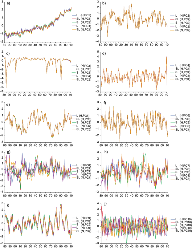
Fig. 5 Rotated principal components of global and hemispheric sea, land, sea and land temperatures, WMGHG, TRF, AMO, SOI, NAO and PDO. 

The next five principal components (PC2-PC6) are highly correlated (≥ 0.95) uniquely to one of the physical variability modes included in the analysis and to STRAT. The second mode of variability (PC2) corresponds to PDO for all temperatures and datasets. STRAT is represented by PC3 for L ^H and SL ^N , PC5 for SL ^H and S ^H , and PC4 for L ^N , while NAO is represented by PC4 in all cases with the exception of L ^N , in which case this mode corresponds to PC3. AMO corresponds to PC3 in SL ^H and S ^H and in all other cases this mode is represented by PC5. SOI corresponds to PC6 in all cases. PC7 (PC8 in the case of L ^H ) and PC8 (PC7 in the case of L ^H ) represent modes of variability that difficult to identify, but which do not correspond to the natural modes included in the analysis. Although PC7 and PC8 probably reflect part of the differences in how the CRU and NASA adjust and process data, the strong similarity of these modes across the different datasets suggests that PC7 and PC8 may also represent true natural variability modes. PC9 closely corresponds to solar variability and PC10 mainly represents unstructured noise.

The features of the common warming trend represented by PC1 are relevant to better understand the observed response of the climate system to increases in radiative forcing. The existence of a current slowdown in the warming - and its causes - are of particular interest to the scientific and policy-making communities and the general public. For this purpose, we apply the Perron-Yabu test to investigate the existence of structural breaks in the slope of the trend function of the first principal components that were extracted. The estimated break dates are compared to those found in the radiative forcing variables as a simple way to establish the existence of co-breaking.

Consistent with what has been reported earlier (^{Estrada et al., 2013}b; Estrada and Perron, 2016; ^{Kim et al., 2017}), TRF and WMGHG are characterized by two highly significant breaks in the slope of their trend function. These breaks occurred at the same time in 1960 and in the early 1990s and, by construction, the breaks in TRF are mainly imparted by WMGHG. As can be seen from Table VIII, the first principal components for the various series are also characterized by two breaks in the slope of their trend function. In all cases, the first break is significant at the 1% level and most of the break dates are concentrated around the mid-1960s, similar to the breaks found in the radiative forcing series. The 95% confidence intervals of the break dates confirm that the dates for the first break in the PC1 series are not statistically different between them nor are they different from that of TRF. Similarly, the dates for the first break in the PC1 series are not statistically different to that of WMGHG, with the exception of PC1(L ^H ), the PC1 that corresponds to the set involving land temperatures from CRU. Even in this case, the difference in the break dates is just a few years. This common break between temperature series and radiative forcing occurring in the 60s marks the onset of global warming dominated by anthropogenic factors (Estrada et al., 2013b; Estrada and Perron, 2016; Kim et al., 2017).

Table VIII Tests for the existence two breaks in the slope of the common trend between temperature and radiative forcing series. 

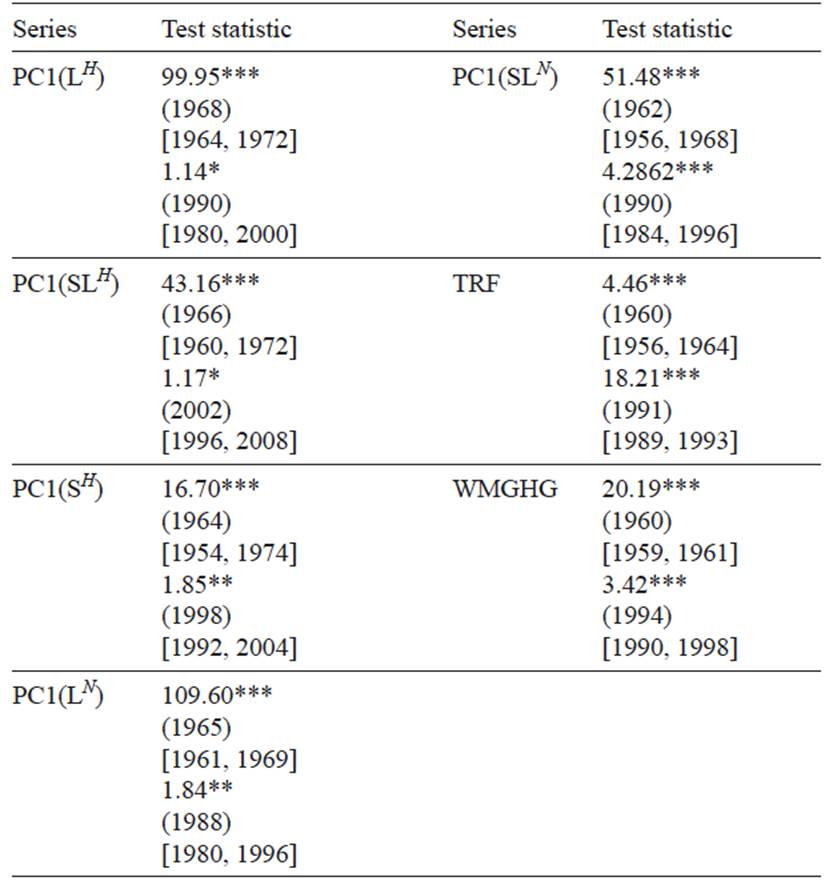
The main entries are the values of the PY test. ***,**,*, denote statistical significance at the 1, 5 and 10% levels, respectively. The estimated break dates are given in parentheses and their corresponding 95% confidence intervals are shown in brackets.

The PC1 and radiative forcing series are also characterized by a second break occurring during the 1990s. In all cases, the break in the slope of the trend function in the PC1 series is significant at the 5% level, with the exception of PC1(L ^H ) and PC1(SL ^H ) for which the breaks are significant at the 10% level. The estimated break dates for all PC1 series are not statistically different from those of WMGHG and TRF. The exceptions are PC1(SL ^H ) and TRF, for which the 95% confidence intervals do not overlap. The presence of this common break occurring in the 1990s provides strong evidence for the existence of a slowdown in the warming and allows, at least partially, to attribute it to the anthropogenic interventions with the climate system. According to ^{Estrada et al. (2013}), the current slowdown in the warming is mainly imparted by the decrease in the rate of growth in the radiative forcing of CFCs and methane that resulted from the adoption of the Montreal Protocol and from changes in agricultural production in Asia, as well as by the increase in atmospheric aerosols emissions (^{Velders et al., 2007}; ^{Montzka et al., 2011}; ^{Kai et al., 2011}; ^{Hansen et al., 2011}).

A two-compartment climate model (^{Schwartz 2012}) is useful to understand the physical model behind the empirical results offered in this paper. The upper compartment is composed of the atmosphere and the upper ocean and it is characterized by a small heat capacity and short time constant to reach its equilibrium state. The lower compartment represents the deep ocean and has a high heat capacity and a long time constant to reach its steady state. These compartments are thermally coupled. When a positive and sustained external forcing is imposed, the upper compartment temperature increases, leading to changes in the absorbed/emitted radiation at the top of the atmosphere and to a heat flow to the lower compartment. The analysis and results presented in this paper pertain to the response of the upper compartment of the climate system to changes in radiative forcing. The TCR, represented by γ in (4), is characterized by the short time constant of the upper compartment. As mentioned in the previous section, TCR relates time dependent changes in temperatures to time dependent changes in radiative forcings given by T(t) = S _tr F(t),where S _tr is the TCR. Over the observed period, the response of the climate system to the forcing has been determined by the time to reach the steady state (usually referred to as the time constant) of the upper compartment and the TRC. This provides a physical explanation of why global and hemispheric surface temperatures share the same nonlinear trend and the same features of the radiative forcing, and of why surface temperatures rapidly adjust to changes in the radiative forcing (Schwartz 2012; ^{Estrada et al., 2013}b).

6. Conclusions

This paper highlights the need to distinguish between the observed temperature trends and the underlying warming trends when investigating the response of the climate system to changes in external forcing. Due to the effects of natural variability, which distorts the underlying trend, investigating the trends and features of observed temperatures as a substitute for investigating those of the underlying warming trend can be severely misleading. Conclusions based on characterizing the trend in observed temperatures, instead of that of the underlying trend, can hardly be useful to shed light on issues such as the existence of a slowdown in the warming or how the ITA has changed.

Although several factors have an effect over the fitted trends in global and hemispheric temperatures, our analysis strongly suggests that their underlying trend and its features are imparted by the radiative forcing. Furthermore, the common trend between radiative forcing and temperature series, and its features, can be substantially attributed to human activities. This conclusion is strongly supported by the cotrending analysis and the characterization of the extracted common trend. One of the most debated features of the warming trend is the existence and causes of a slowdown in the warming since the 1990s (^{Tollefson, 2014}, ²⁰¹⁶). Here, we provide additional empirical evidence showing that the slowdown is a common feature present in the radiative forcing series as well as sea, land, and sea-land temperatures, both at the hemispheric and global scales. As suggested by ^{Estrada et al. (2013}a), the slowdown in the warming has, at least partly, a human origin. According to our results, natural variability has made it more difficult to detect the current slowdown. It is important to note that, even if other factors may have a role in explaining the slowdown in observed temperatures, the results we report here are directly related to the response of temperatures to changes in external forcing and therefore cannot be dismissed as natural variability phenomena.

ITA has been proposed as an emerging indicator of climate change for which a rapid response to changes in external forcing has been detected in the late 1960s (^{Friedman et al., 2013}). Changes in ITA related to external forcings are of particular interest given their potential effect in displacing the intertropical convergence zone, with the implication that the current precipitation patterns over large parts of the world could change (^{Broecker and Putnam, 2013}; ^{Seo et al., 2016}). However, our analysis shows that, although there is a trend in ITA that can be traced to changes in anthropogenic forcings, the structural break in the level and the slope registered in the late 1960s is very likely the product of combining low-frequency variability of different magnitudes, phases and periods that are contained in the temperatures of the northern and southern hemispheres. The difference in the transient response between hemispheres is about 0.054 ºC per W/m². Although this estimate is within the CMIP5 range, it would produce substantially lower increases in ITA than the average of the CMIP5 ensemble. However, it is important to consider that regional forcing factors (e.g., tropospheric aerosols) can have a large influence over ITA and changes in the emissions of these factors can lead to larger temperature contrasts between hemispheres. Given the large effects of natural variability over ITA, our results suggest that this variable may not be a good indicator of climate change.

The results in this paper provide additional evidence supporting the fact that temperatures can be better represented as trend stationary processes with structural breaks in their trend function. The results obtained using new techniques and approaches that are robust to the type of data generating process, such as those presented here, and the broad agreement shown by most attribution studies, make a very strong case supporting the attribution of climate change to human activities. The present study and those of ^{Estrada and Perron (2016}) and ^{Kim et al. (2017}) aim to extend the current focus of observation-based attribution studies to further characterize the warming trend. This can help to provide academic research and policy making with more relevant information about the observed response of the climate system to changes in external forcing.