


 nueva página del texto (beta)
 Inglés (pdf)
 Artículo en XML
 Referencias del artículo
 Enviar artículo por email
 Citado por SciELO
  Similares en
SciELO
Similares en
SciELO 
 Permalink
1. Introduction
For more than a century, climatologists have addressed the characterization of climate patterns using classification methodologies or systems associated with global, regional or local geographic areas. These systems are useful for basic and applied research and diverse usages in a variety of human activities. Classification systems by Koppen (1936), Holdridge (1947, 1967), Trewartha (1968) and Thornthwaite (1948) have been among the most known and used. As our research uses climatological data from Mexico to perform a concept proof of our proposed methodology, the work by García (1964) is a relevant reference because it is a reputed adaptation of Koppen's system for the particular case of the Mexican climatology.
In the second decade of the 21st century, the characterization and representation of climate patterns is a relevant research question. Reasons for this are: (1) The need to understand global climate phenomena, including climate change and its social, economic and political impacts; (2) the availability of vast databases containing climatological data, observed or from reanalyses; (3) the availability of techniques and software tools for data analysis and modeling that use statistics or machine-learning approaches.
The climate is a phenomenon that does not depend on political division borders; however, with this in mind, the general approach in our research involves a reverse perspective: how to discover and to represent the patterns that characterize political division units from their climatological features. This also involves the relationships or similarities among these units based on common climatological characteristics. Figure 1 shows the 32 political units of Mexico. The primary motivation to address the climatological characterization of these units is that the detailed knowledge of climate patterns that are associated to specific political units is highly useful not only to climate researchers, but also to public policy makers and to private company strategists. This is even more relevant if the climate change phenomenon and the necessity to develop new public policies are considered. For instance, a policy maker in the agriculture department of a state could match the need of crops dictated by markets, but neglected in this region, with the plants suitable for the climate of his state, to favor their cultivation. A pharmaceutical manufacturer could modify the containers shipped to certain states, based on their environment.

On the one hand, the most known climate classification systems define climate types depending on climatological features (e.g., rainfall and temperature) and, eventually, other non-climatological features, such as biome. Then, the climate types are associated to specific territories on a map or a spatial database. However, the general approach in data mining consists in the discovery of patterns from analysis of the values of a series of features, usually without considering previous models of the data in the particular domain. We can solve our particular problem using automatic classification algorithms, mainly trees. In addition to characterizing the territorial units from specific climatological values, it is possible to identify, trace and analyze the aggregation (and disaggregation) patterns of these groups, by using relatively simple rules that show thresholds and differences among the values of climatological variables. In general terms, this research is feasible because; (1) there exists a considerable amount of climatological data from Mexico; (2) there exist some automatic classification algorithms that are available in commercial or free software; and (3) the authors are knowledgeable in fields such as climatology and data science.
The paper has the following divisions: Section 1 defines the research problem, delimitates its scope and describes the research approach. Section 2 presents related work in the area of climate classification systems. Section 3 discusses works on the application of automatic classification algorithms in the climatology and meteorology areas. Section 4 gives a theoretical background on automatic classification trees. Section 5 presents our methodology. Section 6 describes the experimental data used to develop and evaluate our method. Section 7 presents the empirical results obtained by applying the method to the experimental data. Section 8 discusses the results and suggests potential applications of the methodology and the results, and Section 9 presents the conclusions and suggests future research work.
2. Problem definition
The research problem is to develop a methodology that characterizes and represents the climate patterns of subnational political division units (e.g., states, provinces, departments) based on observed monthly temperatures and rainfalls, by exploiting the advantages of automatic classification algorithms. In this research, a climate pattern is the combination of climatological features (i.e., monthly maximum and minimum temperatures and cumulative rainfall) and their respective specific values associated with a determined political division unit (particularly, states). The reason for focusing on these climatological features is that they are the most frequently analyzed in the most used climate classification systems (e.g., Koppen, Holdridge, Thornthwaite, etc.). Therefore, they are the variables most commonly recorded by climatological stations worldwide and during long periods. Very often, these data are available as long and complete time series with acceptable levels of reliability. Although other climate classification systems analyze other different or additional features, this research work constitutes our first approach to the problem; therefore, simplicity is a constraint to test our methodology. Other climatological features can be incorporated in future work.
This research considers subnational units of political division because public policy makers need information on climate (and climate change) focused on their respective geographical scopes. Since the beginning of the XXI century, an accurate knowledge of the local environment, its patterns, and its variability is highly useful to decision-making in local governments and diverse industrial sectors. Therefore, in addition to global and regional climate classifications, subnational and local classifications have been introduced, for instance, Garcia (1964), which are easier to understand to non-expert users and easier to exploit in areas different from climate science.
The usually applied procedure to characterize climatologically territorial units of political division consists in overlapping, either visually or mathematically, a political division map of the area of interest on a climate classification map. In other words, a climate classification system and its corresponding geographical representation on a map (or on a spatial database) are previously required for the task. The climate classes or typologies in the selected classification system depend on the climatological data used to produce the typology. It may happen that those data and the resulting typologies can be obsolete or inaccurate to characterize a particular territory on a given period. Thus, some the most known climate classification systems need occasional revision or adaptation to specific areas, for instance, the adaptation of Koppen's system for the Mexican environments by Garcia (1964). The obsolescence or inaccuracy can be larger due to the global climate change phenomenon.
The scope of this research is delimitated to implement an experiment in which a dataset containing climatological features from a collection of climatological stations in Mexico is fed into an algorithm ofthe supervised machine-learning paradigm. The climatological features are monthly maximum and minimum temperatures and cumulative rainfalls. Although available, no other features were used because Koppen (1936) and Garcia (1964) focused only on these, and due to our previous experience in Mexico's climate. The algorithm to produce classification trees is J4.8 (Witten and Frank, 2000), also known as J48, which is the WEKA implementation of the C4.5 algorithm. This algorithm is selected because: (1) classification trees are easy to understand to non-experts of the machine-learning area, and (2) implementations of this algorithm are available in a wide variety of software toolkits, either commercial or free.
The particular approach of this research involves using a supervised machine-learning algorithm as a means to discover and to represent patterns that exist in climatological data that pertain to the specific political divisions of Mexico. The purpose is not to use the produced models as tools for automatic prediction or forecasting of the territorial unit (e.g., state) associated with a set of climatological features, but instead to use the models only as representations of the climatological patterns. The target attribute is the name of the political division unit (i.e., the state) corresponding to the location of every climatological station. As the state is a known data that is available in the dataset, there is no need for using the models to predict this nominal value.
For a dataset, classification trees can automatically discover and represent the rules that constitute a particular climatological pattern, including the hierarchies and interactions among the variables and their threshold values The intent is that this methodology can be applied to the climatological characterization of political division units of any country, using a similar collection of climatological features.
3. Climate classification systems
A climate classification system is a set of arithmetical and logical rules, and simple tags or labels that identify and define specific climate types based on climatological and, eventually, other complementary features. Most of these classification systems have been created to characterize the climate of large regions of the world, and these areas are associated to the major world biomes. Then, the systems are adopted and adapted on more specific territories; for instance, Koppen (1936), Holdridge (1947, 1967), Thornthwaite (1948) and Trewartha (1968). Most of the world and regional climate maps have used Koppen's classification, which uses monthly temperatures and rainfall as climatological features to classify the climates. At present, these maps are updated and used to show changes in climate depending on climate change scenarios. The systems underwent some revisions and adaptations. For instance Belda et al. (2014), Kottek et al. (2006), and Rubel and Kottek (2010) have used recent climatological data of the second half of the 20th to produce updated classifications based on Koppen.
In the particular case of Mexico, three climate classification systems are adopted and widely used: Koppen, Holdridge, and Thornthwaite. In García (1964), a remarkable adaptation of Koppen's classification appears. In general terms, she used a procedure that is similar to Koppen's, but she introduced a series of new climatological types, subtypes, and variants. García's system is now used in Mexico since several decades ago, not only in climatology but also in other sciences, such as biology and agriculture.
4. Application of machine-learning algorithms to climatology and meteorology
Machine-learning algorithms have been applied to the climatology and meteorology fields for the last three decades, at least. The most used algorithms in these areas are artificial neural networks (ANN) and unsupervised clustering. The application of classification trees seems to be recent and infrequent. Regarding ANN, they are used in the modalities of self-organizing map (SOM), multi-layer perceptron (MLP) and neuro-fuzzy. See for instance, Badr et al. (2014), De Oliveira et al. (2009), Hewitson and Crane (2002), Jiang et al. (2012), Kisi and Shiri (2014), Robinson et al. (2013), and Shank et al. (2008). Cavazos (1999) applies SOM to the study of extreme precipitation in Northeastern Mexico. Clustering is used, for instance, by Bankert et al. (2009), Bravo-Cabrera et al. (2012), and McGuire and Tang (2013). Lu and Qin (2014) use a combination of ANN and clustering. Celik et al. (2014) use association rules, and Tavakol-Davani et al. (2013) use classification trees. Two very interesting works on the application of automatic classification trees are Zhang et al. (2013a, b), who use J4.8, the same tree generator algorithm used in our work, to model tropical cyclone rainfalls (see Fig. 2).
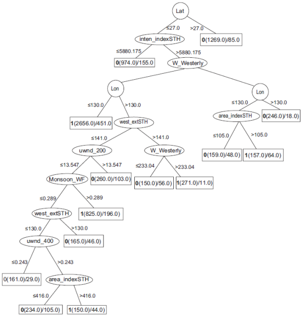
Fig. 2 An example of a classification tree (reproduced from Zhang et al., 2013b) that classifies a cyclon into 0 ("does not make a landfall along the Chinese coast") or 1 ("makes a landfall..."). These numbers are seen to the left of the left parenthesis in each leaf node (rectangles in the tree). Lat is the latitude; inten_indexSTH is the intensity index of the subtropical high, W_Westerly is the westerly index; lon is the longitude; area_indexSTH is the area index of the subtropical high. West_extSTH is the westward extension index; uwnd_200 is the zonal wind in the 200- hPa layer; Monsoon_WF is the monsoon index; uwnd_400 is the zonal wind in the 400-hPa layer, and area_indexSTH is area the index of the subtropical high.
In turn, Faghmous et al. (2014) address the application of data science to the research of climate change. Coria et al. (2013) successfully use J4.8 to characterize political division units, particularly municipalities, from a demographical perspective addressing the digital divide phenomenon in Mexico. After a review, to our knowledge, no related work addresses the climatological characterization of territorial units of political division by using automatic classification algorithms.
5. Theoretical background on automatic classification algorithms
A reputed reference on data mining and automatic classification algorithms is Han et al. (2005). Classifying consist in assigning a class (a label) to an object, based on a set of its features. For instance, in Zhang et al. (2013a, b), the labels "makes a landfall along the Chinese coast" or "does not make a landfall along the Chinese coast," are assigned to tropical cyclons, based on their latitude, minimum central pressure, 10-min maximum sustained wind speed, etc. A classifier is an algorithm that implements classification. A supervised classifier is built by giving it a set of objects, each one with its right class. The algorithm discovers or learns what combination of features indicates what class. This construction phase is also known as the learning or training phase of the classifier, considered as a parameter tuning that is done by the classifier without human intervention. After training, a test phase is performed to measure the accuracy of the classifier model. After this, the classifier is ready to classify new objects: to assign a class to each one. The accuracy of a classifier is the ratio of correct classifications; e.g., a classifier that makes 12 mistakes when classifying 100 objects has an accuracy of 88%, where accuracy is equal to the number of objects correctly classified, over the number of total objects to be classified. The Kappa coefficient (Cohen, 1960) is another way to gauge the goodness of a classifier, defined as: Kappa = [ace - Pr] / [1 - Pr], where acc is the accuracy, and Pr is the probability that the classifier assigns a right class randomly. It is more robust than simple percent agreement (between the machine classiier and the reality) because it takes into account the agreement occurring by chance. Other measurements, like recall, precision, and F-measure are also used to evaluate a classification model quantitatively.
When performing a model test, recall, precision and F-measure are computed for each class. Recall is the rate of true positives of a class. Recall (e) = correct classifications of stations to state e/number of stations in state e. Precision is the proportion of cases that truly are of a class divided by all classified into that class. Precision (e) = correct classifications of stations to state e/number of stations classified as e. High precision means the classifier had many more correct assignments to e than incorrect ones; high recall implies that the classifier classified most of the stations belonging to e as e. For state e, F-measure (e) = [2 x Precision (e) x Recall (e)]/[Precision (e) + Recall (e)]. These three indices measure the model's skill is to recognize instances of a class. Then, the weighted average of F-measure is the average of all F-measures, each weighted according to the number of cases with that particular class label. Thus, the weighted F is an overall measure of the model goodness.
There are many types of supervised classifiers. The tree-based classifiers make their decision procedure understandable to a person, which is an advantage. Thus, we selected the classifier J4.8 (Witten and Frank, 2000) to analyze our dataset. It is inspired on the reputed C4.5 algorithm (Quinlan, 1993), and it is available in the open-access WEKA data-mining tool (http://www.cs.waikato.ac.nz/ml/weka/), another advantage.
The J4.8 algorithm is a generator of classifier trees. The input to the tree is an object to be classified. This object travels down the tree, selecting at each node of the tree a branch, according to the value of the feature that the node evaluates. For instance, if the first node of the tree assesses a cyclone latitude, then the input object will go to one of the branches less than or equal to 27 degrees, or greater than 27 degrees (see Fig. 2), according to its latitude. In each subsequent node, a different test (usually on a different feature, for instance the intensity index of the subtropical high) is tried. The last node, a leaf, outputs the class of the object (for example, does not make a rainfall along the Chinese coast). The tree is available for examination by the user, yet another advantage. Every branch, from the root to a particular leaf, constitutes a classification rule (if-then rule). A rule has two parts: antecedent, and consequent. The antecedent (the if part) is the collection of comparisons (i.e., features with associated values) represented from the root through the node before the leaf. The consequent (the then part) is the leaf representing a class (a political division unit). Section 8.4 shows some rules. Figure 2 is an example of a classification tree.
The construction of the tree depends on a set of samples (in our case, weather stations) labeled with their corresponding states. The tree is binary; each node has two branches or none (leaf node). A leaf node is one at which all the samples have the same label (they belong to the same state). If an unknown station "falls" into a leaf, it is assigned the state of the leaf.
A non-leaf node splits the objects to be classified according to the attribute of the node. The attribute and the value at which the split is produced are selected so that the normalized information gain (difference in entropy) is greatest. The left and right branches are treated as smaller trees, and the algorithm is recursively applied to them. A branch is split unless it is a leaf node or no more variable-value pairs remain. In this case, the expected value of the label is assigned to the leaf node. For instance, if 75% of the samples falling into this node have label Oaxaca, and 25% have label Chiapas, and there are no more tests possible, then the expected value is Oaxaca.
The J4.8 classifier produces binary splits for numeric data, as most tree classifiers do, allowing the same variable to be used "partially," permitting other variables to be tested and contribute to the decision, if they provide more information gain. Thus, the same variable can appear at different tree levels on a given branch. On the other hand, it is possible to construct a tree classifier with multiple splits when testing a variable, for instance, the KD-tree classifier (Guzman, 1995). In a given branch, it tests a variable just once. Due to its inability to use the same variable at several levels on the same branch, it is, in general, less accurate than a binary tree.
6. Methodology
Based on data mining techniques, the following general steps should be followed as a methodology:
i. Determine the political division unit to be used as target attribute (e.g., state, department, province) for the interested country.
ii. Retrieve monthly climatological data from the source databases: 12 maximum temperatures, 12 minimum temperatures, and 12 cumulative rainfalls to conform the 36 features for each climatological station previously selected. The name of the political division unit of every station must be available, to be used as a target. All these data constitute the initial dataset.
iii. Check data quality considering missing values, outliers, or bias. The recording period should be continuous (i.e., no missing values for several consecutive months) and their minimum duration should be 30 years, to ameliorate the effects of periods of unusual climate. Allow missing values (the algorithm permits this), but a long sequence of them has a negative influence on the accuracy of the results. Make the initial and ending years of periods as similar as possible among the periods. Discard values beyond two standard deviations (outliers). Bias in the measurements was ignored in our case (it was too difficult to check).
iv. Rounding of numbers in climatological features (i.e., no decimals) is recommended to avoid the production of unnecessarily detailed models.
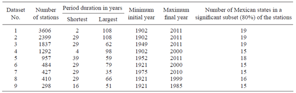
v. Perform descriptive statistics analyses (histogram, column diagram, and Pareto) on these features: period durations, beginning and ending years, and political division units. In our case, data selection (step vi) and feature selection (this step) were as follows. For data selection, the 5329 climatological stations in the UNI-ATMOS database ((Fernández-Eguiarte et al., 2014; refer to section 6) were reduced to 3606 by eliminating stations with too many missing or incomplete time series, although stations with periods less than 30 years were included. Of course, we did not remove a significant percentage of stations from any political unit (a compressed plot of these 3606 stations appears in Fig. 3). This yielded our initial dataset (Dataset 1 in Table I), from which another eight groups of meteorological recordings were formed, each of them representing a distinct epoch (Datasets 2-9). The sizable recording period was a relevant aspect; thus, removing stations with less than 29 years of recording produced Dataset 2. Considering the starting time of recording yielded Dataset 3, which encompasses the second half of the 20th century, while Dataset 4 comprises the whole 20th century. Dataset 5 is Dataset 3 considering long recording periods, that is, longer or equal to 39 years. Dataset 9 includes short periods, at least of 16 years. Datasets 6, 7 and 8 show variations on durations, initial and final years. These datasets underwent descriptive analyses, but they were not used to discard any of them. Instead, all nine datasets were used to produce classification trees, whose results are shown in section 7.
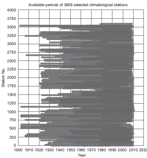
Fig. 3 Visualization of the periods corresponding to stations whose data are available in complete time series of at least 2 yrs. with all monthly data for maximum and minimum temperatures and cumulative rainfall. The vertical direction has been compressed to keep it to a reasonable size.
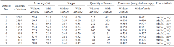
Table I Statistical description of the nine experimental datasets to produce classification models (the total number of Mexican states is 32).
With respect to feature selection, it was not made by hand. Instead, the J.4.8 algorithm makes this selection automatically (from the dataset fed to it), placing those features with the largest discrimination power near the root ofthe tree (Witten and Frank, 2000), using entropy considerations. Section 7.2 shows the most discriminant features thus selected. Section 7.1 covers the best trees (for Dataset 2) where these features appear, in fact, near the root. vi. Different subsets of stations can be considered to produce other datasets from the initial dataset, if different durations of periods or different initial and ending years in periods exist. In addition, the climate change phenomenon can be considered, and a particular year defined as the boundary to create different datasets (e.g., data before the year 1950, and after that year).
vii. Produce a classification tree model for every dataset by using the J4.8 algorithm (the WEKA software is recommended).
viii. Evaluate the trees quantitatively, analyzing the values of accuracy, Kappa, and F-measure. Aim to achieve an accuracy of at least 70%, which will provide confidence that the method produces reasonable results. For instance, in our case, the probability of a random assignment of a state to a station being correct is 1/32 (since Mexico has 32 political units). More accurately, it is at most 0.12, which is the ratio of the surface ofthe largest state, Chihuahua, to the whole surface of Mexico.
ix. Interpret, evaluate and determine the theoretical soundness of the best tree from the climatology perspective.
x. Extract and assign identifiers (e.g., integer numbers) to the classification rules in the best tree.
xi. Group the rules corresponding to every political division unit.
xii. Rank the rules in every political division unit based on its support value (i.e., the number of stations meeting each rule).
7. Experimental data
The experimental data in this research are organized as a series of datasets obtained from the UNIATMOS database (Fernandez-Eguiarte et al., 2014), which contains data from 1902 to 2011. However, the available periods of data records are not equal among all stations. UNIATMOS was created and updated by using daily data from the Servicio Meteorológico Nacional (Mexican Weather Service. SMN). It contains 5227 climatological stations with maximum temperatures, 5225 stations with minimum temperatures, and 5320 stations with cumulative rainfalls. Among other data, it includes 36 yearly climate features per station (from January to December) as follows: 12 features of maximum temperature, 12 features of minimum temperature, and 12 features of cumulative rainfall. Station ID, latitude, longitude, altitude, station name, municipality, and state constitute data on every station. The state is the political division unit used as the target in the classification tree models. Climatological stations were placed in Mexico at different times and by various authorities. Budget played a role, too. Thus, they are not uniformly distributed (Table II gives the number of stations per state). Nevertheless, since states generally have smaller budgets, their distribution tends to be somewhat balanced.
Statistical representativity is an essential aspect when producing analyses and models in climatology and data mining. Therefore, differences in the durations and initial and ending years of periods of climatological stations in the database are considered, to produce a first dataset (Dataset 1). According to the methodology, values of climatological features (and altitude) were rounded to integers. Altitude is included in the dataset but only to determine its contribution to the classification process. Temperature is in degrees Centigrade, cumulative rainfall is in millimeters, and the altitude is in meters above sea level.
Other eight alternate datasets were produced from Dataset 1 by selecting different subsets of stations. Table I presents the statistical description of all the nine datasets. There are important reasons to use nine different datasets: (1) durations, initial, and final years of recording periods of stations are heterogeneous; (2) climate change influences the climate patterns corresponding to the late 20th and early 21st centuries. The nine experimental datasets of this research are available at: http://tinyurl.com/gq6dc73.
The original database of 5320 weather stations was reduced to 3606 in Dataset 1 by eliminating stations with missing or incomplete time series, although stations with periods less than 30 years were included. Dataset 2 is a subset of Dataset 1 that only contains stations having periods of 29 or more years. Dataset 3 is a subset of Dataset 2 that focuses on the second half of the 20th century and the beginning of the 21st century (1949-2011). The climate in Mexico during the first half of the 20th century is different from that of recent decades, which would reflect climate change according to the Intergovernmental Panel on Climate Change (IPCC). Dataset 4 focuses on the whole 20th century (1902-2000) and includes stations with short periods (four years as a minimum). The year 2000 is selected conventionally as a time boundary, supposing that patterns before this year are different from those after. Dataset 5 is similar to Dataset 3 because both are focused on the second half of the 20th century and the beginning of 21st, but Dataset 5 uses only periods greater than or equal to 39 years. Datasets 6-8 are also variations on the durations and initial and final years of the periods; Dataset 9 includes short periods (the minimum length is 16 years).
The last column in Table I shows the number of Mexican states in a significant subset (80%) of the stations. It is computed by performing a Pareto analysis on the state name in every dataset. The analysis calculates the cumulative relative frequency of stations, and counts the states. The purpose is to verify the representativeness of states in every dataset. Considering that the total number of Mexican states is 32, they are suitably represented in every dataset, as Table I shows.
Since the number of stations per state is not the same, this introduces certain bias. Nevertheless, we preferred not to delete any station, since this amounts to discarding useful information.
8. Results
8.1 General aspects
Table III summarizes the results of 18 models (nine with the altitude attribute and nine without it) that the J4.8 algorithm produced on the nine datasets. Two trees are created for each dataset: one that includes the altitude feature as one of the predictors, and one that does not. All these models are available at: http://tinyurl.com/zctyjqa. The reason to produce 18 models is that comparisons between their accuracies, Kappas, quantities of leaves, and F-measures are necessary to identify advantages and disadvantages in each case. The quantity of leaves refers to the number of terminal nodes in a tree.
In the literature, there is no unanimity regarding the acceptance criteria in the evaluation of classification trees because this depends on the particular domain and purpose of the models. However, it is clear that an accuracy much larger than that produced by a random assignment should be attained; the closer to 100%, the better.
According to Table III, the trees with highest accuracies, Kappas and F-measures are the two which were produced using Dataset 2 (containing 2399 climatological stations). The effect of using the altitude feature as one of the predictors is only marginal, although consistent: in eight of the nine models, accuracies increase 1 or 2 percentage points, at most, and Kappas increase by 0.01 or 0.02 units. In turn, the quantity of leaves in the trees does not present a consistent or significant effect. As altitude is not strictly a climatological feature, the tree that does not include altitude is selected as the best model. This tree and its corresponding numbered rules can be downloaded from: http://tinyurl.com/zeoytgd. Its accuracy, Kappa, and F-measure are 60.5, 0.59, and 0.604%, respectively. These results are lower than our desired goal (point viii of the methodology section), but still acceptable, in our opinion.
Dataset 2 is the most efficient to produce the models due to these possible reasons:
It includes long enough periods whose duration is at least 29 years.
Its minimum initial year is 1902 and its maximum final year is 2011, respectively, which offers almost all of the available historical scope.
Climate homogeneity or heterogeneity of a state with respect to its size is immaterial to our study, since our unit of analysis is the meteorological station (and not the political unit). Therefore, the result is given according to how stations are grouped by the parameters that the classifier considers, independently of the size of the state, or how close a station is to another station in a contiguous state. According to the map in Figure 4, there is a climatically defined area occupying two complete states, BCand BCS. In addition, an entire state (Son) and three-quarters of another state (Chih), or several states (Mex, Hgo, Pue, Tlax, Qro), definitely have different climate from the first two ones.
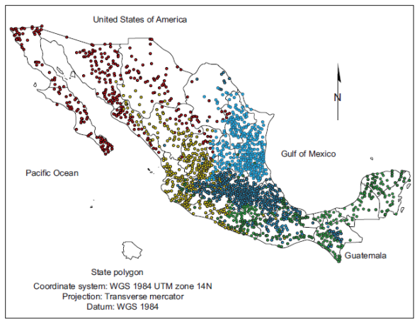
Fig. 4 The four basic climate patterns based on the features with highest discriminant capability at the top two levels in the best tree (from Dataset 2 with 2399 stations). Each point is a climatological station. Light blue: May rainfall > 26 mm and Jan max temp ≤ 26 °C. Dark green: May rainfall > 26 mm and Jan max temp > 26 °C. Light orange: May rainfall ≤ 26 mm and Jan rainfall > 50mm. Intense red: May rainfall ≤ 2 6mm and Jan rainfall ≤ 50 mm.
8.2 The most discriminant features
The root is the feature located at the top node of the tree model. This feature is important because it has the highest classification capability; i.e., it contributes most to the classification process. In seven of the nine trees, the root is rainfallmay (cumulative rainfall of May) (see Table III). The root of the other two trees is rainfalljun (cumulative rainfall of June), relevant from the Mexican climatology perspective because May is the month in which the rainy season begins in Mexico, and June is the second month of this season. In the best tree (http://tinyurl.com/zeoytgd), rainfall may is also the most discriminant feature; its threshold value is 26 mm. The second most discriminant features are rainfalljun (threshold: 50 mm), and maxtempjan (maximum temperature of January, threshold: 26 °C). January is usually the coldest month in Mexico. Therefore, in general terms, this model expresses that the two major aspects considered to characterize the political division units are: rainfall at the beginning of the rainy season and maximum temperature in the coldest month.
As the best tree is the corresponding to Dataset 2, the map in Figure 4 presents its 2399 stations and the most general climate patterns discovered and represented by that tree. The number of description rules in a tree is equal to the number of its leaves (329 in this tree). However, the deepest leaves usually describe a very low number of instances, indicating that those patterns are not highly frequent. Therefore, the most general (i.e., most frequent) patterns are those that are described by features with the highest discriminant capability, which are located at the highest levels in the tree (i.e., the root and the features that are nearest to it). Thus, the feature at the root (May rainfall) splits the 2399 stations into two branches (i.e., two subsets): those greater than 26 mm, and those less than or equal to 26 mm. If the two highest levels in the tree are considered (May rainfall, Jan max temp, and Jan rainfall), then four collections of stations are identified. If three or more levels are considered, then eight, 16, 32, etc. collections can be identified. Therefore, the four most general climate patterns are:
May rainfall > 26 mm and Jan max temp ≤ 26 °C (light blue)
May rainfall > 26 mm and Jan max temp > 26 °C (dark green)
May rainfall ≤26 mm and Jan rainfall > 50mm (light orange)
May rainfall ≤ 26 mm and Jan rainfall ≤ 50mm (intense red)
This is interesting because the spatial distribution of the four patterns can be clearly visualized on the map: light blue is located at the center and the east, dark green is at the south and south-east, light orange is at the west, and intense red is at the north-west.
8.3 Characterization of the Mexican states
Every Mexican state can be characterized by selecting and grouping all its leaves from the best classification tree (http://tinyurl.com/zeoytgd) and joining them using the OR logical operator. Therefore, 32 groups of OR-joined rules describe the climatological profiles of all the Mexican states. Sorting the rules by support value in every state group is recommended so that the most supported rules of the state are presented first. These groups and the sorted rules can be downloaded from: http://tinyurl.com/hl4gzcr. The comprehension (and user friendliness) of a rule is enhanced if the user, on a first reading, "simplifies" it by ignoring its branches with small support. See in this regard section 8.4.
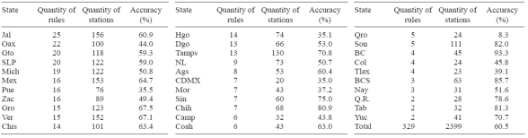
Table II presents the quantity of rules per state in the best tree (http://tinyurl.com/zeoytgd). The four states with more rules are: Jal (25), Oax (22), Gto (20) and SLP (20), and the 3 states with fewer rules are Q.R. (2), Tab (2) and Yuc (2). It contains, in addition, the classifier accuracy by state. The number of rules per state depends, mainly, on two aspects: the quantity of climatological stations in the state, and the diversity of climates in that state. As an example, the detailed characterization of two states are presented below:
State = Tlax: IF
rainfall_may > 26, max_temp_jan ≤ 26, max_temp_jul ≤ 29, rainfall_apr > 20, rainfall_jan ≤ 35, rainfall_aug > 97, min_temp_jan ≤ 5, rainfall_jan ≤ 13, rainfall_may ≤ 81, rainfall_Jan > 5, min_temp_Jan ≤ 4, rainfall_apr > 34, rainfall_aug > 99, rainfall_dec ≤ 8, min_temp_jun ≤ 9 (9 stations, 1 exception) [rule R183]
or
rainfall_may > 26, max_temp_jan ≤ 26, max_temp_jul ≤ 29, rainfall_apr > 20, rainfall_jan ≤ 35, rainfall_aug > 97, min_temp_jan ≤ 5, rainfall_jan ≤ 13, rainfall_may ≤ 81, rainfall_jan ≤ 5, min_temp_may ≤ 8 (5 stations, no exception) [rule R170]
or
rainfall_may > 26, max_temp_jan ≤ 26, max_temp_jul ≤ 29, rainfall_apr > 20, rainfall_jan ≤ 35, rainfall_aug > 97, min_temp_jan ≤ 5, rainfall_jan ≤ 13, rainfall_may > 81, rainfall_jun ≤ 196, max_temp_nov ≤ 22, min_temp_jul ≤ 9, max_temp_mar > 23 (5 stations, 1 exception) [rule R189].
or
rainfall_may > 26, max_temp_jan ≤ 26, max_temp_jul ≤ 29, rainfall_apr > 20, rainfall_jan ≤ 35, rainfall_aug > 97, min_temp_jan ≤ 5, rainfall_jan ≤ 13, rainfall_may ≤ 81, rainfall_Jan > 5, min_temp_Jan ≤ 4, rainfall_apr ≤ 34, rainfall_feb ≤ 9, min_temp_jul ≤ 11, rainfall_jul ≤ 159, rainfall_may > 64, rainfal_jan ≤ 10 (4 stations, no exception) [rule R173].
State = BCS: IF
rainfall_may ≤ 26, rainfall_jun ≤ 50, rainfall_may ≤ 8, rainfall_jun ≤ 2, min_temp_oct > 13, max_temp_aug ≤ 38, rainfall_apr ≤ 3, rainfall_jun ≤ 1 (58 stations, 1 exception) [rule R2]
or
rainfall_may ≤ 26, rainfall_jun ≤ 50, rainfall_may ≤ 8, rainfall_jun ≤ 2, min_temp_oct > 13, max_temp_aug ≤ 38, rainfall_apr ≤ 3, rainfall_jun > 1, min_temp_jan ≤ 9 (4 stations, 1 exception) [rule R3]
or
rainfall_may ≤ 26, rainfall_jun ≤ 50, rainfall_may ≤ 8, rainfall_jun > 2, rainfall_sep > 121, max_temp_jan ≤ 25 (3 stations, no exception) [rule R15].
8.4 Rules with highest support
The most significant rules in a classification tree are those with the highest support. Support is the number of climatological stations that are described by the antecedent of the rule. A law can present exceptions, i.e., stations that meet the antecedent but do not meet the consequent (do not belong to that state). Confidence of a rule is the ratio of instances (stations) in that rule that match its antecedent and in fact belongs to the state designated by the rule, divided by the total numer of stations that just match the antecedent. From the best tree (http://tinyurl.com/zeoytgd) the rules with the highest support are identified and presented in Table IV with their respective confidence values. All sorted 329 rules can be downloaded from: http://tinyurl.com/jxo5gul, with their support. The two first rules of Table IV are shown below (R2, the third rule, was already presented above with the other rules for BCS):
R9: IF rainfall_may ≤ 26, rainfall_jun ≤ 50, rainfall_may ≤ 8, rainfall_jun > 2, rainfall_sep ≤ 121, min_temp_dec > -1, min_temp_jan ≤ 8 THEN Son (91 stations, 2 exceptions). Support of R9 is 91/2399=3.8%, since 91 stations out of the 2399 fall into R9; confidence of R9 is 91/(91 + 2) = 0.978 = 97.8%, since two of these 91 stations do not belong to Sonora.
R196: IF rainfall_may > 26, max_temp_jan ≤ 26, max_temp_jul ≤ 29, rainfall_apr > 20, rainfall_jan ≤ 35, rainfall_aug > 97, min_temp_jan ≤ 5, rainfall_jan > 13, rainfall_jun > 115, rainfall_dec ≤ 19, rainfall_jul ≤ 275, min_temp_jun ≤ 11, rainfall_feb ≤ 14 THEN Mex (67 stations, 8 exceptions).
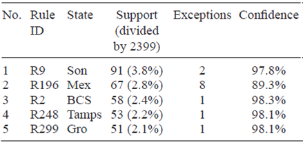
If the support of a rule is among the highest of the tree, then that particular pattern is among the most frequent in the dataset and, particularly, in that specific state. For instance, R9 describes a climate pattern that is typical of Sonora (Son), a dry territory with cold winter, and R196 describes a typical pattern of the State of Mexico (Mex), with rainy summer and cold and wet winter.
8.5 Confusion matrix
The confusion matrix is automatically produced in the test phase of the model. It shows the confusion of the model while classifying the stations into states. Figure 5 shows the confusion matrix of the best tree.
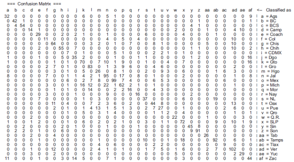
It is a square (n x n) matrix, where n is the number of Mexican states. An item in the array tells how many stations were (correctly or incorrectly) classified into a state. Each row represents a state. A column represents the classification determined by the model (i.e., classified as). The sum of every row is equal to the total number of stations of a state.
A number on the diagonal gives the quantity of correctly classified stations regarding a particular state. For instance, the model determined that 32 stations belong to Ags, which is true (see the item in the first row and first column). Every number that is out of the diagonal represents stations classified into a wrong state. For instance, number six at the first row and eleventh (k) column represent stations that the model considers belonging to Gto, when they really belong to Ags. This matrix is interesting because it suggests that most of the confusions occur among climatological stations that belong to neighbor states; for instance, in the first row, stations of Ags are confused with those of Gto, Jal or Zac (see map in Fig. 1).
The sum of all values along the diagonal represents the total quantity of correctly classified instances (i.e., true positives); therefore, the difference of the total number of stations in the dataset minus the real positives is equal to the number of incorrectly classified stations. An ideal although very unusual confusion matrix would present values greater than 0 along its diagonal only, and equal to 0 in any other position. WEKA uses the confusion matrix to compute automatically true positives, true negatives, false positives and false negatives. In turn, these are used to calculate accuracy, Kappa, recall, precision, and F-measure.
9. Discussion and suggested applications
The empirical results in Table III show that the models offer accuracy in the classification of climatological stations into states that are greater than or equal to 0.46 (the worst cases are Datasets 8 and 9) and less than or equal to 0.60 (best cases, Datasets 1 and 2). A naive baseline can be obtained by a random assignment of a given weather station to a state. The probability of this assignment to be correct is at most 0.12, as stated in step viii of section 6. Moreover, this work does not seek to find where to place a meteorological station in certain state. The stations were installed along many years by different government agencies. For this analysis, those stations fulfilling certain criteria were selected, as pointed out in the methodology section.
A series of the most significant patterns in the Mexican climate identified by the tree models are:
May rainfall is the feature with the highest capability for discrimination of states, which is consistent with theories and systems using this as a critical piece of information. It determines the beginning of the rainy season in Mexico.
The particular value of 26 mm for the May rainfall determines a threshold to classify the states.
The next two features with highest discrimination capability in the best tree are June rainfall (threshold: 50 mm), and maximum temperature of January (threshold: 26 °C), involving summer rains and the coldest month, respectively.
Robust patterns of states with very typical climate emerge; for instance, dry seasons and cold winter in Son, and rainy summer with cold and wet winter in Mex.
The main reasons for using the J4.8 algorithm are: (1) the patterns are represented as classification rules in the tree branches, (2) these rules are easy to understand, so they are highly useful, and (3) the rules are highly detailed, allowing to describe subtle similarities and differences between pairs of states.
In contrast to the usually applied procedures, our methodology does not depend on any previous climate classification system, but only on observed data. If these data are recent and reliable, the climatological characterization of the territorial units can be more accurate and dependable than the characterization produced by the usually applied procedure. In addition, our methodology is easily used on new observed data as these become available.
The tree models offer a new perspective on the identification and representation of climatological patterns for political division units. Among other aspects, the tree models allow to discover and to represent how similar two given territorial units are. The model uses climatological features possessing discriminant capability, along with their respective threshold values. This combination is able to distinguish between different territorial units.
This work has produced a methodology, a collection of datasets, a series of descriptive statistics analysis, and several machine-learning models that are valuable research products by themselves. They can be applied to other tasks involving analysis, modeling, and visualization. Several applications are suggested below.
The methodology can be used to characterize the climates of the political division units of other countries besides Mexico, for which data on monthly maximum and minimum temperatures, and cumulative rainfall should be available. The minimum duration of periods in the available data should be 30 years, approximately.
The main application of the best tree (http://tinyurl.com/zeoytgd) of the Mexican dataset has been the climatological profiling of the states of this country. The nine datasets correspond to different subsets of climatological stations in the Mexican territory. As the produced datasets consider distinct periods, they can be exploited to perform other statistical analyses and machine-learning models. For instance, attractive models may be created using other algorithms, such as classification rules, multi-layer perceptrons, or clustering. This latter procedure can be used to discover, for instance, a small number of clusters, based on the 36 climatological features.
An application of the best tree model and its corresponding dataset is the production of a new database with one additional feature in which climatological stations are labeled depending on the tree branch (or sub-branch) they belong to. The collection of stations represented in it can split into two, four, eight, 16, or 32 subsets. The number of subsets is a power of two because the tree is binary. Every subset can be labeled with a nominal value, for instance a color, and shown on a map. Figure 4 shows a map with stations in four colors.
Finally, although it can be very unusual, the best tree can be used, with some certainty level, to determine the political division unit where a climatological station is placed, in case that this specific data is not available due to some extraordinary reason.
10. Conclusions and future work
This article has presented a methodology to discover and to represent climate patterns of political division units in a country using monthly maximum and minimum temperatures and rainfalls, by means of automatic classification trees. This methodology assumes that every territorial unit contains at least one climatological station and that the recording periods of stations are similar in their durations and in their initial and ending years. Based on the experimental results, our claim is that the classification tree is a useful technique to discover and represent these patterns, and offers high expressivity to climatologists.
Our theoretical contributions are both from the conceptual and the methodological perspectives. From the conceptual perspective, we formalized a notion of climatological characterization of political division units by means of models using classification trees. In addition, the climate patterns (and their representation) of the political division units corresponding to a specific country (Mexico, in this case) constitute innovative knowledge by themselves. In turn, from the methodological perspective, our proposal offers an effective and original procedure to characterize political division units (states, in this case) by means of their climatological features. In addition, our methodology is different from the most common approaches to this problem because it does not depend on any previous climate classification system (e.g., Koppen, Holdridge, Garcia, etc.), or any map representation of climate typologies.
The strengths of this methodology are, among others, the following:
Climate patterns discovered and represented by the tree models are finely detailed by means of subsets of the 36 climatological features with their respective threshold values.
The most useful features to perform the discrimination are automatically identified by the tree production algorithm (i.e., the most discriminant features are placed at the top of the tree) and, in turn, the least useful features are automatically placed at the bottom or disregarded by the algorithm.
Although the models make some mistakes, these generally occur between pairs of states that either are neighbors or have very similar climates.
The tree models offer a fine granularity that shows the subtle differences that can exist within one single territorial unit or between two territories with very similar climates.
Future research work should address creating analyses and models with this methodology on data from other climatological datasets, either from Mexico or from other countries, considering different features and other scopes of political division units, either larger or smaller. As an improvement to our work with J4.8, it is possible to construct many decision trees and then select the best (the random forest algorithm [RF]). Other automatic classification algorithms could be used; e.g., classification rules or clustering.
An interesting work would be an empirical comparison of the classification results obtained by these classification models vs. those by expert climatologists using the 36 climatological features. Another interesting product can be a map of Mexico showing types of climatological stations as colored points using two, eight or 16 colors, depending on the branches of the best tree, as explained in section 8 and shown in Figure 4. Finally, our analyses and models can be used as preliminary inputs to a more ambitious research work that aims at revising or updating a known climate classification system, for instance, Garcia's system for Mexico.
It is interesting to see how predictability changed with time, analyzing different periods. We left that for a future work, in order to keep our report to a reasonable extention.

