


 nova página do texto(beta)
 Inglês (pdf)
 Artigo em XML
 Referências do artigo
 Enviar este artigo por email
 Citado por SciELO
  Similares em
SciELO
Similares em
SciELO 
 Permalink
1. Introduction
Vehicles are the major agents responsible for the loss of air quality in cities, contributing to 70% of pollution. Notably, vehicles account for 70% of carbon monoxide (CO2), more than 50% of hydrocarbons (HC), and almost 45% of nitrogen oxides (NOx) (Tomassetti, 2005), in addition to other substances containing volatile organic compounds (VOCs), sulfur and microparticles. In the last 40 years many studies have been carried out regarding these agents of pollution, especially in North America and Western Europe (Alcaide López, 2000).
In Argentina, cities such as Capital Federal, Córdoba, Mendoza, Rosario, La Plata and San Miguel de Tucumán are more exposed to the effects of atmospheric pollution due to their increasing population, inappropriate location of industries, low presence of green areas, and a growing vehicle fleet (Petcheneshsky, 1996). The city of Neuquén, together with its surrounding areas, has been characterized in the last decades by its fast growing population and economy, with the subsequent increase in the number of motor vehicles.
Over the last few decades a variety of research studies has been conducted on distinctive cities with high vehicle density. The majority of these studies used quantitative in situ measurements or qualitative estimations by using a number of models. Venegas and Mazzeo (2002) applied an urban atmospheric diffusion model called DAUMOD, which measured the emissions of carbon monoxide (CO) and NOx produced by public transport motor vehicles in the city of Buenos Aires. The objective of the study was to determine the horizontal distribution of pollution originated by these sources of emission.
Alcaide López (2000) analyzed the phenomena of distribution and dispersion in the city of Madrid, Spain through a Gaussian model of dispersion for a specific case of daily traffic with stable atmospheric conditions. This study involved CO, NOx, SO2 and HC and was carried out in 1996.
Gaioli and Tarela (2001) conducted a quantification of atmospheric pollutants produced by motor vehicle parking lots and thermoelectric centers in Buenos Aires between 2000 and 2012. The vehicle emissions were obtained analytically through indirect data by applying the atmospheric impact software SofIA, a computational model for pollutants dispersion, to determine the concentration of pollutants.
Toro et al. (2001) determined hot emissions of CO, NOx, SO2 and VOCs in the traffic of the city of Medellín, Colombia. To carry out their analysis, they developed a model that calculates emissions in cells and generates an average rate per hour.
Tarela and Perone (2002) applied the SofIA Gaussian model of dispersion to calculate concentrations of NOx and PM10 (particles with a diameter of 10 μm or less) in Buenos Aires, Argentina.
Ruiz and Pabón (2002) showed the distribution of average concentrations of CO in levels close to the surface in Bogotá. They documented emissions on the 10 busiest streets of the city. They found that the monthly variability of CO emissions with most adverse effects took place during the months of April and October with values close to 47 000 mg m-3.
Gantuz and Puliafito (2004) designed a model by using a new methodology of the "bottom-up" type. This methodology was used to estimate the spatial and temporal distribution of mobile sources of emissions, based on data obtained through an auto-transported measurement system in order to obtain experimental results in the city of Mendoza.
Sanhueza et al. (2004), made an estimation of vehicle emissions in Santiago de Chile between 2000 and 2005. They used the Mobile 6.2 model developed by the US-EPA.
Charron and Harrison (2005) studied the emissions of PM25 and PM10 in a main street in London, studying the factors that produced more concentration.
D'Angiola et al. (2006) accomplished an annual inventory of CO emissions for motor vehicles in Buenos Aires in 2003, with different spatial resolutions. They took as reference the COPERT 3 methodology for the calculus of emission factors (EF) (Ntziachris-tos and Samaras, 2000).
Yura et al. (2007) analyzed the CALINE4 estimation for PM smaller than 2.5 μηι on a suburban site in Sacramento and an urban site in London. In the suburban site the results were better adjusted to measurements than in the urban case.
Nayeb et al. (2015) evaluated concentrations and emission factors from vehicles in the vicinity of a highway near Tehran, Iran, finding that pollutants experiment an exponential decline in an area of100 to 150 m from the highway.
Venegas and Mazzeo (2009) compared concentrations of CO in the airflow of an urban canyon with values estimated through various dispersion models. Observed data were obtained from hourly scheduled measurements of CO concentrations during a whole year in the interior of an urban canyon in Gottonger Strass (Hanover, Germany) and on the roof of a bordering building.
Represa (2011) applied the model CALINE4 to determine the dispersion of CO produced by mobile sources in La Plata, Argentina. The results showed that the concentration of this gas did not exceed the limits established by regulations.
In the present work, provincial route No. 7 is considered as a lineal source. We used the Gaussian model of dispersion (a variant model of CALINE4) to calculate CO, NOx and SO2 concentrations, obtaining data from motor vehicles in different atmospheric conditions on the surrounding areas of this highway, between the cities of Neuquén and Centenario, Argentina. The studied route is a highway with an important traffic flow that crosses a residential area and a leeward productive area that could be affected by the resulting pollution.
2. Area of study
The area of study included the Neuquén-Cente-nario stretch on provincial route No. 7, which runs through residential areas, an industrial sector, and an agricultural area (Fig 1). Traffic in this area is intensive since Neuquén is an important commercial, administrative and economic center, which also functions as a touristic stop for many travelers during holidays.
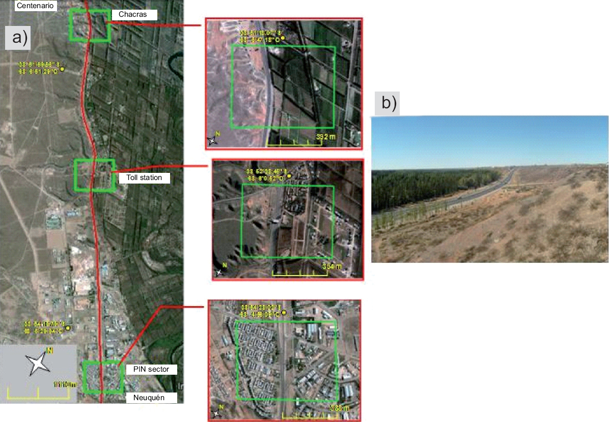
Fig. 1 (a) Satellite image of the Neuquén-Centenario stretch (red line) on provincial route No. 7 (left). The sectors selected for analysis are identified with a green square and amplified to the right: Industrial Park (PIN, bottom), former toll station (middle) and Chacras (top). (b) Photograph of the study area.
The route crosses the edge of the plateau and circulates through the river valley, with a slope of about 50-70 m. The plateau is covered with dispersed herbaceous and shrubby vegetation (Fig. 1), and fruit trees are grown in the valley. Due to differences in the use of soil and the topography of the study area, several sectors were chosen for analysis. Figure 1a shows the areas of study and an illustrative photo of the region (vicinities of the former toll station).
We used traffic data (timetable, type and amount of vehicles) for the period 2004-2009 from the company Caminos del Comahue (toll operator, see Fig. 1), and average traffic data for the same period from the Provincial Highway Department and the Provincial Department of Statistics and Census. We also used meteorological data form the Neuquén station of the Servicio Meteorológico Nacional (Argentine National Meteorological Service).
3. Methods and sources of information
Gas emissions were calculated with COPERT3, a computer program used to calculate emissions from road transport which classifies vehicles into categories and subcategories (type of gas, weight of vehicle, size and technology of the motor, etc.) (Ntziachristos and Samaras, 2000), and also with the air quality dispersion model CALINE4 (Benson, 1992).
Dispersion and concentration of CO, NOx and SO2 were analyzed in the Industrial Park (PIN) and Chacras sectors, as well as in the former toll station (Fig. 1). Four months were selected as representatives for each season of the year: March (autumn), July (winter), October (spring), and December (summer). An average working day was established for each month to estimate the emissions in three representative hours: 08:00, 12:00, and 18:00 LT.
Emission factors were calculated according to vehicle categories, type of motor, age of the vehicle fleet, and current regulations in Argentina. Natural gas vehicles (NGV) were not considered. It was assumed that traffic flow was homogenous in each area of study. In general, the traffic flow increased at an average annual rate of 8.1% during the study period. The months of January, March, July and December showed the highest increases in traffic density.
On a weekly basis, traffic decreased considerably during weekends. On working days peaks were recorded at 08:00 and 18:00 LT, with averages of 1337.0 ± 18.0 vehicles/h at 8:00 LT, and 1376.0 ± 68.0 vehicles/h at 18:00 LT.
Figure 2 shows the traffic behavior during three working days in 2009, discriminated by daylight hours. From 07:00 to 20:00 LT the traffic flow exceeded 800.0 vehicles/h, and from 23:00 to 05:00 LT it was less than 400.0 vehicles/h.

Fig. 2 Hourly traffic for three working days during the year 2009. N: number of vehicles circulating through the former toll station. Traffic data were provided by the company Caminos del Comahue.
On average, for the three representative days in 2009, 91.0% of the traffic consisted of cars and minivans, 7.0% of vans, and 2.0% of buses. The proportion of vehicles according to the type of gas was based on the Enterpreneurs Asociation of Motorvehicles Manufacturers (ADEFA) database (2006), Giacobbe et al. (2007) and Ravella et al. (2006), assuming that 90% of the automobiles were powered by gasoline and 10% by diesel; and of the utilitarian vehicles, 60% were powered by gasoline and 40% by diesel.
Traffic speed was estimated based on field observations subjected to the sector and vehicle category. For the PIN area, it was estimated at 80.0 km h-1 for cars and utilitarian vehicles and 60.0 km h-1 for vans and buses. In the toll sector, it was estimated at a maximum of 60.0 km h-1 and a minimum of 20.0 km h-1 for all categories. Finally, in the farming sector, estimated speed was 100 km h-1 for cars and utilitarian vehicles and 70.0 km h-1 for vans and buses.
Atmospheric stability was estimated by using the empiric classification of Turner and Pasquill (Pasquill, 1961; Turner, 1964) enumerated from 1 to 7 (1: extremely unstable; 2: moderately unstable; 3: lightly unstable; 4: neutral; 5: lightly stable; 6: moderately stable; 7: extremely stable).
Figure 3 shows the relative frequency of atmospheric stability for the four months that represent the seasons of the year in three different hours of the day. Neutral stability was dominant. In morning hours during spring, summer and autumn, lightly unstable situations were predominant in contrast to more stable ones in winter. Near noon a tendency toward unstable situations was observed, especially in warmer months as compared to winter.

Fig. 3 Relative frequency (f [%]) of atmospheric stability in Neuquén as a function of the month at (a) 08:00 LT, (b) 14:00 LT and (c) 20:00 LT, for the period 1959-1991. Classes: 1: extremely unstable; 2: moderately unstable; 3: lightly unstable; 4: neutral; 5: lightly stable; 6: moderately stable; 7: extremely stable (source: Ministerio de Energía y Minería [Ministry of Energy and Mining of Argentina]).
The height of the mixed layer was calculated in different hours of the day through the simplified method, which uses data of insolation, wind velocity and atmospheric stability (Spadaro, 1999). This data was compared to the monthly relative frequency at 20:00 LT published by the Ministry of Energy and Mining (see Fig. 3) for 1959-1991 in Neuquén. Thirty receptor points were selected for each area. (see Fig. 4a-c).
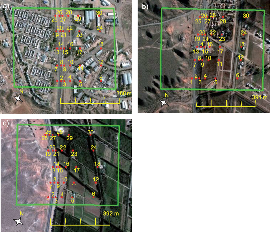
Fig. 4 (a) PIN sector, (b) former toll station and (c) Chacras sector with the selected receptor points.
The AQRoads model, based on CALINE4, was used to calculate hourly emissions of pollutants (CO, NOx and SO2) (Enviroware, 2004). In this model, the pattern of the traffic flow is defined by a combination of links. For atmospheric simulation, initial data were wind velocity and direction, mixed layer height, and atmospheric stability classes, according to the classification of Pasquill and Gifford (Enviroware, 2004).
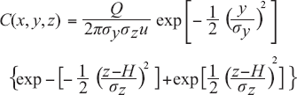
The semi-empirical formulation of the model for a lineal Gaussian source, when the x axis is directed on the same direction as the wind, can be expressed as (Hanna et al., 1982):
 1
1
where C(x, y, z) is the concentration in the point (x, y, z) (μg m-3); Q is the rate of continuous emissions (g s-1); σy (m) and σζ (m) are the standard deviations of the Gaussian concentration distributions vertically and laterally, respectively, and are functions of the downwind distance (x) and atmospheric stability; u is the average velocity of the wind (m s-1) in the direction of the x axis; H is the effective height of the emission (m) (h [height of the emission duct] + AH [height of the plume]); z is the height above the ground (m); and y is the perpendicular distance to the direction of the wind (m) (Hanna et al., 1982).
The model assumes that there are stationary meteorological conditions all over the area, an x axis in the direction of the wind, a flat surface, and that the effects of turbulent diffusion are negligible in comparison to the horizontal transport by the wind. This method excludes conditions of absolute calm.
4. Results and discussion
Moderate and critical conditions of wind flow within the area were calculated. Figure 4 shows the concentration of CO in a transect of the area of study, located between the points 14 and 17 (Fig. 5). Windward receptors (left margin of the route) showed insignificant levels of gas concentrations.

Fig. 5 Monthly and hourly mean concentration (C) of CO m-3) in points 14, 15, 16 y 17 at the (a) PIN sector, (b) former toll station and (c) Chacras sector during March (M); July (J); October (O), and December (D).
The highest concentrations of gases were found in all cases in the nearest point to the traffic flow (point 14). Surprisingly, we found a gradual decrease of CO concentrations windward of the route, specifically in the east sector, at 08:00 LT, even though the highest traffic density was observed at 18:00 LT. A possible explanation for this could be that velocity and temperature of the wind are higher at 18:00 LT on this location, causing more turbulence and gas dispersion, as well as lower levels of immission.
A relative maximum of gas concentration was found in all cases at the points 15, 16, and 17 during the months of July and December, both at 08:00 LT (point 14). The maximum traffic density was detected in December at 18:00 LT with a mean of 1548.71 vehicles/h. However, gas concentration was lower at this time. This can be associated with higher wind velocity (10.6 m s-1) and air temperature (27.7 °C).
During October around noon (12:00 LT) a notorious decrease of gas concentrations was observed for the three sectors. CO concentrations exhibited similar values for the sectors PIN and Chacras (with greater velocities), and higher values in the former toll station, reaching levels up to 274.1 μg nT3 in the closest point to the route. In December, NOx concentrations were found to be similar for all sectors and schedules. SO2 concentrations exhibited higher values in point 14 at 08:00 LT, reaching 1.5 μg m-3.
Considering mean concentrations in the closest and farthest points to the route (which are 140 m apart), the highest concentrations of CO and SO2 during the four months were found at the former toll station, being 75% lower in the PIN area, with intermediate values at Chacras (~70% less than in the former toll station, see Figs. 5 and 6). These differences were greater for CO, since CO emissions increase with low speeds.

Fig. 6 Monthly mean concentrations (C) of CO, NOx and SO2 in points 14 y 17 for each sector during March (M), July (J), October (O), and December (D).
NOx concentrations were 14% higher in the Chacras area during the four months, with similar values in the PIN sector and the former toll station, which may be due to the higher speed of vehicles, which favors a higher emission of NOx. In all sectors, greater concentrations of all gases were detected during July (~20% more than during March and October in areas close to the route and 45% in distant points) and December (~15% and 7%, respectively, Fig. 6).
During July 2009, gas concentrations were higher in comparison to the rest of the months, reaching points located farther from the route, while in December the ratios diminished with the increase in distance to the route. This situation could be due to the mixing layer height, which reached its minimum in July (200-560 m) making the dispersion of gases difficult, and its maximum in December (560-800 m). In addition, wind speed was lower in July (ranging from 2.6 to 3.9 m s-1) in contrast to December, when values were between 2.3 and 10.6 m s-1.
The spatial distribution of concentrations was also calculated (Figs. 7-10) (8,9) comparing opposing situations due to differences in wind speed, mixed layer height and vehicle speeds. The first case comprises situations with wind speeds of 2.3 m s-1 (Fig. 7a) and 10.6 m s-1 (Fig. 7b) during December at 08:00 LT, exhibiting areas with much higher concentrations in the vicinity of the route.

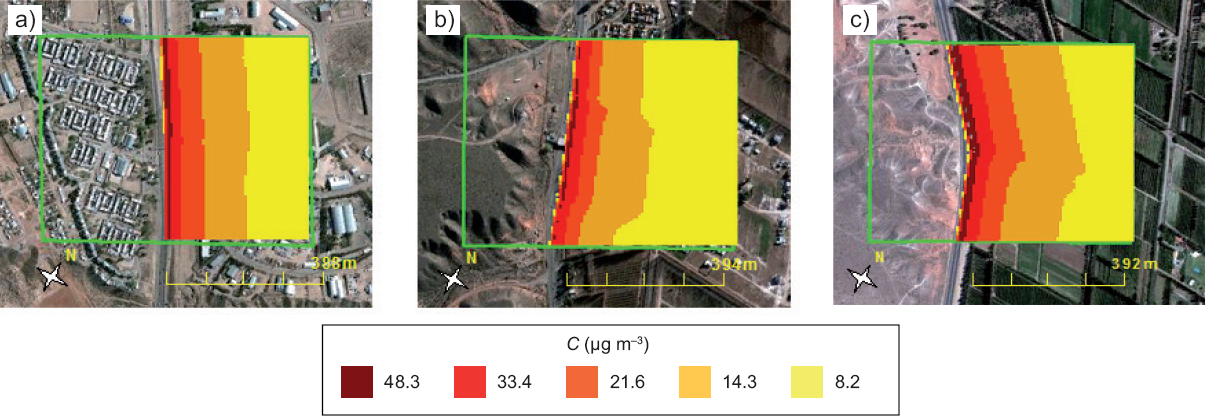
Fig. 8 Spatial distribution of the NOx concentration (C) (in μg m-3) during July at 08:00 LT in the (a) PIN sector, (b) former toll station, and (c) Chacras sector.
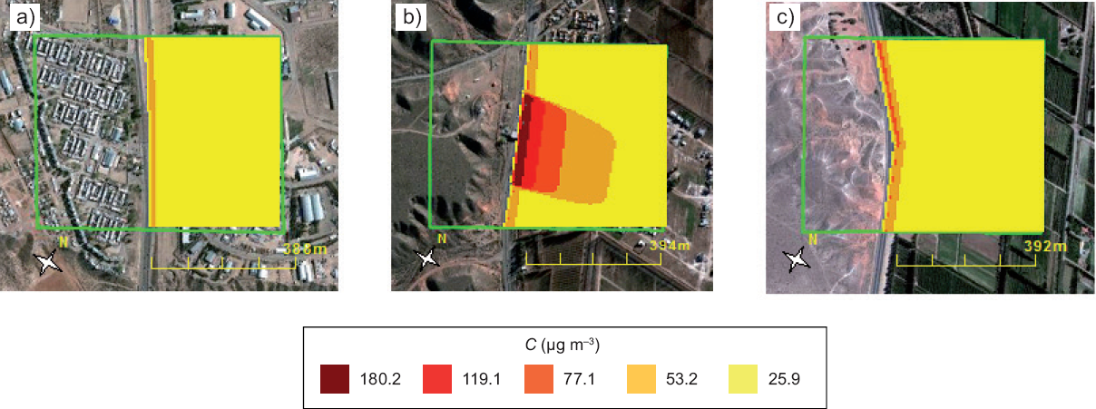
Fig. 9 Spatial distribution of the CO concentration (C) (in μg m-3) during July at 08:00 LT in the (a) PIN sector, (b) former toll station, and (c) Chacras sector.
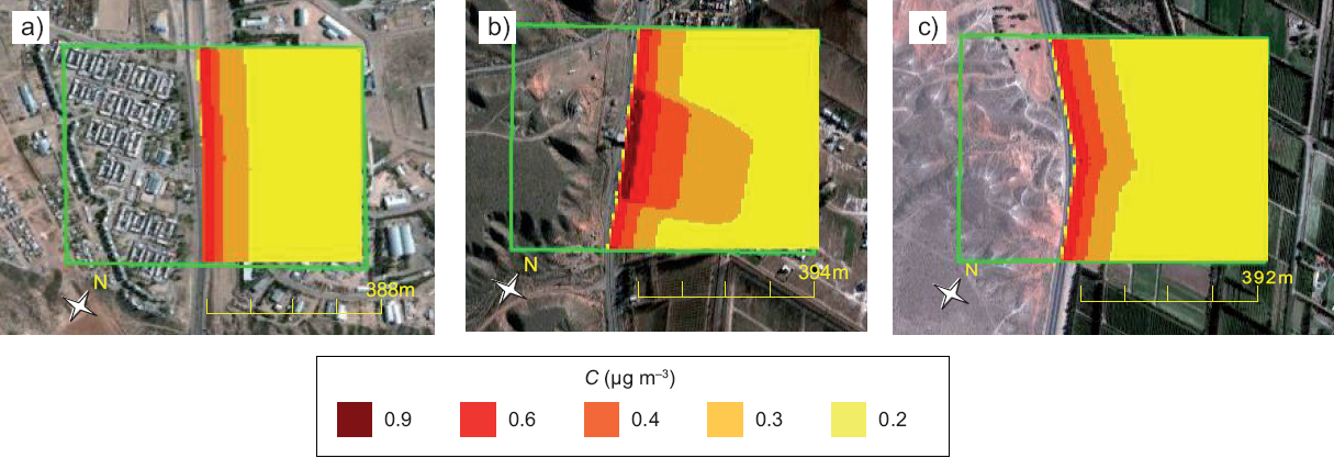
Fig. 10 Spatial distribution of the SO2 concentration (C) (in μg m-3) during July at 08:00 LT in the (a) PIN sector, (b) former toll station, and (c) Chacras sector.
In situations with intense wind there is a higher dispersion and therefore lower gas concentrations. In the nearest leeward area to the route we found an SO2 concentration three times higher with smaller wind intensity. In none of the cases SO2 values exceeded those established by national or international regulations (Argentine law 20284: 2620.0 μg m-3; European Union (EU) standards: 350.0 μg m-3).
Figure 8 presents the spatial distribution of NOx considering that vehicles circulate at higher speeds in the Chacras sector (Fig. 8c), intermediate speeds in the PIN sector (Fig. 8a) and lower speeds in the former toll station (Fig. 8b) during the same day and schedule. In situations that mainly differ regarding vehicle speeds, NOx concentrations were found to be from 26.0 to 55.7 μg m-3 in the first 50 m leeward in all three sectors, and then decreased progressively to 5.0 μg m-3 (yellow area in the figure). The area near the route in the Chacras sector showed the highest concentration of NOx (55.7 μg m-3) due to the increase of emission factors caused by the high speed of vehicles. The measured SO2 and NOx levels did not exceed the values established by national and international regulations (Argentine law 20284: 846.0 μg m-3; EU and WHO standards: 200.0 μg m-3 [OMS, 2005]).
The spatial distribution of CO is shown in Figure 10 (see also Table I).The results indicate a higher concentration of CO in the former toll station (from 147.5 to 212.8 μg m-3 in the area close to the route [30 m leeward of the emission zone]) in comparison to the Chacras and PIN sectors, where emissions did not exceed 90.0 μg m-3, mainly due to different traffic flow speeds in those areas, since the CO emission factor increases with lower speeds. The highest concentrations did not exceed the limits established by national and international regulations (Argentine law 20284: 57 250.0 μg m-3; WHO standards: 30 000.0 μg m-3 [OMS, 2005]).
Table I NOx concentration (C) (in μg m-3) during July at 08:00 LT in the PIN sector, former toll station, and Chacras sector, and maximum concetration according to Argentinean and European Union regulations.
The analysis of pollutants dispersion in the three studied sectors during July at 8:00 LT showed that concentrations were higher in the former toll station, reaching S02 values of 0.8 to 1.2 μg m-3 in the vicinity of the route and of 0.5 μg m-3 at a distance of 200 m, while in other sectors this contaminant did not surpass a distance of 100 m. This higher concentration of S02 in the former toll station could be due to the fact that the emission factor for this molecule increases with the decrease of vehicle speed. Similar to previous cases, the concentrations of S02 did not exceed the limits established by Argentine Law 20284 (2620.0 μg m-3) or EU regulations (350.0 μg m-3).
In the analyzed cases, the meteorological variables with greater influence over concentration values were wind speed and mixed layer height. These results are consistent with the literature (Alcaide López, 2000).
The highest concentration of pollutants was detected along the route because emissions are generated on this highway and are dispersed leeward.
5. Conclusions
NOx exhibited the highest values among the analyzed pollutants, with estimated concentrations that rose up to 33.0% of the limit established by WHO (0MS, 2005) and the EU (measured in the Chacras sector during December at 08:00 LT, with very unfavorable conditions).
Concentration levels were higher in July as compared to December, despite the fact that traffic is 16% higher in December. This maximum in July was probably related to greater pollutant dispersion due to a greater intensity of the wind. In the months considered, conditions at 8:00 LT were favorable for higher concentrations of gases in the surface, coinciding with a lower intensity of the wind. The former toll station area showed higher concentrations of C0 and S02, associated with the decrease of vehicles speed.
It must be considered that emission factors used in this study could underestimate emissions of older cars, since they are more adequate for the newest models (Gantuz and Puliafito, 2004; D'Angiola et al., 2006). Besides, it must be mentioned that analysis of starting and braking characteristics was not taken into account in the former toll area.
As of 2011, the toll station was eliminated due to a regional legislation. This led to environmental benefits for this sector, since there was a significant reduction in the concentration of gases emitted by vehicles as a result of an important decrease in traffic jams.
In days with easterly winds the most affected area was the PIN sector. The highest concentrations of pollutants within this area were found in Parque Industrial, a neighborhood located next to the route where more sensitive receptors were placed. Although the concentrations found in this analysis did not exceed critic values, it is recommended to take samples of the crops located in small farms adjacent to provincial route No. 7 for estimating possible deposits of contaminants in fruits and other associated risks for human health.
Control measures for the maintenance of engines and exhaust gas systems are also needed to keep emissions low. Programs such as the "Technical Inspection of Vehicles" that is applied in Argentina, and improvements in the public transport system would be useful to maintain adequate conditions of air quality.
Even though field data were not accessible for evaluating our results, the literature suggests correlations > 0.83 in estimations made with CALINE4. Levitin et al. (2005) evaluated the model results with data obtained from a study in Finland, and the hourly predictions of N0x at two distances from the road (17 and 34 m), each of these at two heights (3.5 and 6 m), showed correlations of 0.83 to 0.92. The performance was better at 34.0 m. On the other hand, results had worst correlations with lower wind speeds and for wind directions parallel to the route. Ganguly and Broderick (2008) found a reasonable level of agreement between the CALINE results and measurements based on graphical and statistical analysis. Ganguly et al. (2009) found that the model was in good accordance to in situ measurements.
Broderick et al. (2005) validated the model for CO with results within ± 50% of the measurements. These authors specified that the cases with less agreement between model and results were observed in stable situations with low wind intensity. It must be mentioned that these cases, though present, are not frequent in our area of study.

