


 nova página do texto(beta)
 Inglês (pdf)
 Artigo em XML
 Referências do artigo
 Enviar este artigo por email
 Citado por SciELO
  Similares em
SciELO
Similares em
SciELO 
 Permalink
1. Introduction
Circulation in the Gulf of Mexico (GoM) is, to a large extent, dominated by the extension of the Loop Current (LC) and the detachment of anticyclonic Loop Current eddies (LCEs) (Leben, 2005).
The LC extension can be classified, in a broad sense, in two modes. In the retracted mode, the LC penetrates through the Yucatan Channel (YCh) and flows out directly through the Florida Straits. In the extended mode, the LC penetrates further north into the GoM, turning toward the Florida Straits and forming an anticyclonic bulge that irregularly separates as an LCE. The LCEs have a diameter of 200-400 km and a vertical extension of 800-1000 m (Hamilton et al., 2015). They can detach and reattach from the LC several times before their final separation and subsequent migration to the west coast of the GoM occurs (Oey et al., 2005; Chang and Oey, 2010).
LC dynamics and LCE shedding statistics are highly variable and their irregular behavior has been linked to several physical processes such as frontal cyclones, flow instabilities, interactions with topography, transport variations, westward eddy propagation, and Caribbean eddies. In this study, we will explore the sensitivity of the LC and LCE shedding to some of these mechanisms using a numerical model, so we briefly review some relevant results.
Cyclonic eddies along the periphery of the LC, known as Loop Current frontal eddies (LCFEs), are thought to play an important role in the LCE detachment and final separation process (Cochrane, 1972; Schmitz, 2005; Le Henaff et al., 2012). The LCFEs acronym is used generically to identify cyclonic perturbations along the rim of the LC but they may not all have the same characteristics and sources. "Typical" LCFEs have a diameter of 80-120 km and they can be 1000 m deep or more (Vukovich and Maul, 1985; Rudnick et al., 2014). Their origin, intensification, and merging have been linked to LC instabilities, interaction of the flow with topography and coastally trapped waves along the GoM (Chérubin et al., 2006; Oey, 2008; Le Henaff et al., 2012; Jouanno et al.,, 2016). LCFEs appear both on the western LC edge at the Campeche Bank (Zavala-Hidalgo et al., 2003; Oey et al., 2005; Schmitz, 2005) and on the northern and eastern LC edge down to the Tortugas Bank and west Florida shelf (Fratantoni et al., 1998). Slowly evolving cyclones generated on the Campeche Bank can block the penetration of the LC into the GoM and delay the LCE shedding (Zavala et al., 2006). Schmitz (2005) draws attention to the "necking down" process of LCE shedding which involves two cyclones (one on the Campeche Bank and another one on the west Florida slope) moving towards the center of the LC finally producing the shedding.
LCE detachments have also been linked to the interaction between the LC and mesoscale eddies coming from the western Caribbean Sea (WCS). Athié et al. (2012, 2015) present observational evidences of the connection between cyclonic perturbations entering the GoM from the Caribbean and LCE separation events. The impact of these external perturbations in triggering LCE separations, relative to locally generated instabilities over the Campeche Bank, is presently unknown.
Other mechanisms not related to instabilities and LCFEs have been brought to explain the LCE shedding. Using a reduced gravity one layer model for an inflow-outflow problem, Pichevin and Nof (1997) (see also Nof, 2005) show that to conserve zonal momentum, the southern inflow must split into a steady branch that exists to the east along the coast and a northward flowing branch that produces a bulge that grows and is periodically shed (due to the beta effect). They suggest their theory applies to the flow at YCh, so neither instability nor topography are then required to produce a growing LC and LCE sheddings.
Chang and Oey (2010, 2012, 2013) use these ideas to explain the LCE separation in their model. They find a strong positive correlation between LC extension, YCh vorticity and transport consistent with Pichevin-Nof's framework. When the LC bulge is large and YCh transport suddenly decreases, conditions are set for an LCE separation since the inflow cannot arrest its westward tendency for translation due to the beta effect. In Chang-Oey's model there is an asymmetric semi-annual cycle in YCh transport attributed to variations of zonal wind-stress over the Caribbean Sea (CS) with high transports in summer and winter. They suggest this asymmetric transport explains why there is a seasonal preference for eddy shedding at the end of these seasons in their model and apparently in the data as well.
By contrast, Lin et al. (2010) model results have a higher Yucatan transport in LC retracted mode conditions. They only study LC transport fluctuations and link them the topographic from drag, associated to the pressure differences across the ridge in the Florida Straits produced by density anomalies from LC intrusions. Mildner et al. (2013) relate low frequency transport variations to internal variability rather than wind forcing. They suggest that low YCh transport conditions are associated with the position of the LC anticyclonic bulge, which can generate a blocking condition for the flow at YCh.
Besides these different model results, mooring measurements (Athié et al., 2015) do not show such a clear relation among transport, LC extension and vorticity. They suggest high interannual variability and a stronger annual cycle in transport rather than semi-annual.
Several studies have investigated the role of topography on LCE separations. Chérubin et al. (2006) relate the formation of cyclones to the instability of the LC potential vorticity front. Their subsequent evolution is explained by the interaction with topographic features of the Campeche Bank. Oey (2008) associates the formation and evolution of deep cyclones to the instabilities of the LC, which are related to the configuration of the bottom slope in different areas of the Campeche Bank. Le Henaff et al. (2012) emphasize the intensification and vertical alignment of LCFEs when they are advected to the deep northeastern GoM from the shallower northern GoM slope (Mississippi Fan). These intensified LCFEs appear to play a fundamental role in the LCE shedding process.
Despite not being discussed by the authors, the results from both Le Henaff et al. (2012) (their figures 9 and 10) and Oey (2008) (his figure 13) suggest the deep submarine canyon on the eastern Campeche Bank (at around 86° W, 23.5° N) may be a relevant place for cyclone intensification and instability, an issue we address with one of the numerical experiments carried out in this paper.
Our research shares similar objectives to the studies mentioned above, but we investigate the sensitivity of the LCE process and LC behavior with respect to mechanisms not previously considered: the effect of Caribbean perturbations, the smoothing of the model topography (a necessary step in models such as POM and ROMS to avoid a pressure gradient computational error), and the impact of the deep canyon on the eastern Campeche Bank, using different model configurations. Despite the changes, experiments reproduce fairly realistic characteristics of the circulation, such as the sea surface height variability, the vertical structure of the Yucatan and the Loop Currents. All the configurations are capable of producing LCE detachments. However, our study highlights the different statistics of the LCE and LC obtained from the configurations. These differences can be partly explained by the dissimilar LC behavior in the experiments.
It is important to mention that throughout the paper we refer to LCE separation as the condition of final LCE release (i.e., no further reattachments occur) whereas an LCE shedding or detachment indicates the LCE is cut-off from the LC but can reattach again.
The paper is organized as follows: Section 2 describes the configuration of the reference experiment and the different modifications used to build the sensitivity experiments. Section 3 validates the control simulation with observations and highlights similarities and differences with the sensitivity experiments. Results regarding LCE separation statistics and LC metrics are presented and linked to key dynamical aspects of the circulation produced by the experiments in Section 4. Finally, Section 5 contains the conclusions of this work. Two appendices are included for completeness: Appendix A provides a detailed description of the numerical model and Appendix B derives the energy equations and energy exchange terms discussed in Section 4. A movie of the relative vorticity produced by the simulations at two different depths (300 and 1400 m) and some complementary figures are included as supporting material.
2. Description of the reference and sensitivity model configurations
The NEMO model version 3.2 (Nucleus for European Modelling of the Ocean, [Madec, 2008]) is used for the GoM, in a regional configuration, to simulate its circulation, LC dynamics, and eddy shedding features (a detailed description of the model is provided in Appendix A). The model domain (98° W-81° W, 15° N-31° N, Fig. 1) includes the GoM and western CS.

Fig. 1 Model grid and bathymetry (colors in meters). Boxes al and a2 are defined to investigate mean and eddy variability upstream of in the CS and LC area, respectively. Green lines indicate the location of the eastern and southern open boundaries.
The characteristics and main objectives of the different model experiments and their configurations are the following:
EXPERIMENT REF: This is the reference run where the best model parameters and unmodified topography are employed. It is considered to be the most realistic configuration or standard against which all the other experiment results are compared to. Details of the configuration are given in Appendix A.
EXPERIMENT VISCO: This experiment was designed to investigate the impact of Caribbean perturbations on the LC dynamics and LCE separations. Following Jouanno et al., 2008, the model was modified in the CS region by introducing a high viscosity box located at 90.0° W-81.5° W, 15.9° N-20.8° N (Fig. 2a) using a Laplacian operator with a coefficient of 3000 m2s-1. Elsewhere outside the box, a bilaplacian operator with a coefficient of -1.25 x 10¹⁰ m4s-2 is used as in the REF experiment. This substantially damps the amplitude of the eddies in the CS but has a smaller impact on the large scale mean flow.

Fig. 2 The panels illustrate the modifications used in the sensitivity experiments. (a) The gray box indicates the region where viscosity was increased to damp the presence of Caribbean eddies entering the GoM (experiment VISCO). (b) The black line marks the region where the bathymetry was smoothed (experiment SMOOTH, see text for details). The area between the solid and dotted lines is a transition region where the original bathymetry is matched to the smoothed bathymetry by sinusoidal fitting. (c) The box marks the location where a deep submarine canyon is removed from the bathymetry (experiment CANYON).
EXPERIMENT SMOOTH: The goal of this experiment is to test the impact of smoothing the GoM bathymetry on the LC behavior, while maintaining the same topography as for REF upstream of and at the YCh region (Fig. 2b). The region enclosed by the solid box in Figure 2b was smoothed using the average of the bathymetry at the four corner-points surrounding each model grid point. Smoothing the topography just in the LC region intends to evaluate if the modification of small geographical features (e.g., capes, bumps) and reduced topographic slopes can influence the LC behavior and the generation or amplification of instabilities. Topography is not changed at YCh and Florida Straits to keep inflow and outflow conditions similar to REF. It is worth mentioning that our smoothing produces only a 1% volume increase with respect to REF's volume grid, so, in that sense, the bathymetry of both experiments is quite similar.
EXPERIMENT CANYON: In this experiment, the deep submarine canyon located between 86.7° W-85.1° W, 22.7° N-24.6° N (Fig. 2c), was eliminated from the bathymetry. The submarine canyon is a prominent topographic feature, which could play a major role in the intensification of LCFEs as some numerical results suggest (Oey, 2008; Le Henaff et al., 2012).
Main features of each experiment are summarized in Table I.

3. Validation of the model results
Each numerical configuration (REF, VISCO, SMOOTH, and CANYON) is integrated from 1992 to 2009 and their output from 1996-2009 is used for the analysis (i.e., ffour-yr spin-up). We do not carry out a detailed comparison of the simulations with data and among themselves, since the objective here is not to determine which configuration is better but only to highlight basic similarities and differences among the experiments. As shown below, all experiments are able to reproduce the basic features of the circulation in the region, particularly the LC and its eddy shedding (see the movie in supporting material).
Figure 3 shows the standard deviation of the sea surface height (SSH) of each experiment for comparison with AVISO (calculated for the period 19962009, Fig. 3a). AVISO consists of weekly maps of SSH anomalies interpolated on a grid with a spatial resolution of 1/3° using the method of Le Traon and Ogor (1998). All simulations produce a relatively similar and realistic SSH variability with high variability in the LC region, spreading to the western GoM, marking the preferred migration trajectories of the LCEs once they separate from the LC.

Fig. 3 SSH standard deviation (m) for the period 1996-2009 from (a) AVISO and experiments (b) REF, (c) VISCO, (d) SMOOTH, and (e) CANYON. All runs reproduce realistic SSH variability.
The SSH standard deviation of experiment REF in Figure 3b has two maximum cores in the LC region.
The southern maximum is related to the LC extension in the simulation, with high variability on the northeastern corner of the LC, where cyclones tend to intensify (see section 4.2 below), whereas the northern core is related to the LCEs position. Experiments VISCO and CANYON have similar characteristics, while SMOOTH produces a single high variability core within the LC area. Notice also the differences in the extension of the high variability values along the Yucatan slope produced by the experiments.
Another common test for GoM models is their ability to reproduce the observed structure and variability of the flow at YCh. Figure C1 in the supporting material shows the vertical structure of the normal flow at YCh, its standard deviation and the first two empirical orthogonal functions (EOFs) from all experiments, for comparison with observations (Candela et al., 2003) and other model results (Ezer et al., 2003; Chérubin et al., 2006; Le Henaff et al., 2012). All experiments reproduce the mean structure and variability of the flow reported in Sheinbaum et al. (2002) except for the surface Cuban counter-current. In all our simulations, a weak mean northward flow is produced instead, although the standard deviation there is much higher than the mean, as in observations. In addition, the structure of the EOFs and the variance explained is also similar to observed ones (e.g., Abascal et al., 2003) and to the ones obtained in other numerical studies (e.g., Dukhovskoy et al., 2015).
There are certainly some differences in the fields discussed above produced by each experiment, but what we want to highlight here is that they are all relatively minor, and in general terms, in good agreement with observations. More noticeable differences are found in the LC behavior and LCE separations produced by each experiment and discussed in the following section.
4. Results and discussion
4.1 LC metrics, transport through the Yucatan Channel and eddy shedding statistics from experiments and AVISO
A key diagnostic of the circulation in the GoM is the LC behavior and LCE shedding process. To analyze the similarities and differences among the experiments and AVISO in these important dynamical aspects, we use the metrics defined by Leben (2005). It is based on the identification of an SSH contour that marks the core of the LC, which is then used to compute its extension (length) and the longitude and latitude of its maximum intrusion. We chose the 17 cm contour of the model SSH since it coincides with the surface velocity maximum in the model within the LC area (same contour is used by Leben (2005) and Dukhovskoy et al. (2015).
A spatially homogenous steric signal, associated with sea level expansion/contraction due to near surface heating, is removed from each AVISO SSH map by subtracting their spatial average over depths exceeding 200 m in the GoM, before computing the LC metrics and comparing it with the modeling results. This signal does not contribute to the dynamical variability of the LC, but can contaminate the estimation of the LC metrics (Dukhovskoy et al., 2015; Hamilton et al., 2015).
Differences in LC extension and its variability turn out to be very important to understand the experiment results. Figure 4 shows the histograms and statistics of the latitude of maximum intrusion. Similar results are obtained from the other LC metrics (not shown).

Fig. 4 (a) LC metrics histograms of the latitude of maximum intrusion. Ordinates indicate the number of times (as a percentage) the tip of the LC falls within the latitude interval specified in the abscissa. (b) Latitude statistics (median, mean, standard deviation, 1st, and 3rd quartiles) for AVISO and experiments REF, VISCO, SMOOTH, and CANYON during the period 1996-2009. The large-scale steric signal related to near-surface ocean heating has been filtered out from the AVISO data by removing the spatial average of each weekly map.
The SMOOTH experiment has the shortest mean and median LC extension of all experiments, but its standard deviation and quartiles are the largest (Fig. 4b). It is also the only experiment with a more symmetric bimodal (i.e., retracted-extended) condition, as the histogram of LC northernmost latitude shows (Fig. 4a). The retracted mode is centered in the 24.5-25° N bin, and the extended mode is in the 26.5-27.5° N bin.
The LC tends to be more extended in CANYON and VISCO experiments than in REF, but CANYON's standard deviation and quartiles are the smallest of all and, therefore, have a relatively more stable northward extension (Fig. 4a). In these three experiments, the LC is more likely to be in an extended rather than retracted condition (their LC extension histograms are more biased to the right, Fig. 4), with REF having a higher standard deviation in its northern position than VISCO and CANYON. The comparison of the experiments with AVISO suggests that the LC extension in SMOOTH is the most similar to AVISO, but AVISO appears to have a slightly less "bimodal" distribution during the period 1996-2009. Dukhovskoy et al. (2015) show, however, that a longer data record of the Colorado Center for Astro-dynamics Research (CCAR) SSH data does not have such symmetric bimodal distribution, but rather a preference for a more extended state.
Another important diagnostic is the connection between LC extension, LCE shedding and transport variations through YCh (e.g., Chang and Oey, 2013). Monthly averaged volume transports through the YCh for each experiment are plotted in Figure 5a. Whether or not high YCh transports and LC northward extension are strongly and positively correlated is relevant to understanding LCE shedding. Such a relation can vary substantially among different GoM models, as mentioned in the introduction.

Fig. 5 Monthly mean time series of (a) volume transport in the Yucatan Channel (in Sverdrups) and (b) the latitude of maximum LC intrusion (LC metrics) for REF, VISCO, SMOOTH, and CANYON experiments, from 1996 to 2009. Bars indicate ± one standard deviation, showing there is substantial dispersion.
All the experiments produce a clear annual cycle in the YCh transport, with its maximum in June (except for SMOOTH whose maximum is in July) and minimum in November. The open eastern boundary data obtained from the DRAKKAR simulation has a similar transport cycle. Its amplitude is relatively large which leads to a mean YCh transport in the model higher than recently observed in mooring data (Athié et al., 2015).
The average annual transport obtained for REF and VISCO is 35 ± 2.2 Sv. SMOOTH has the lowest seasonal transport, with an annual average equal to 34.6 ± 2.2 Sv whereas CANYON exhibits the highest mean transport (35.4 ± 2.4 Sv). These differences are relatively small. Transport at YCh includes northward and southward flows so it can be influenced by the LC dynamics and other adjustment processes, and it is not expected to be the same in all the experiments.
Monthly averages of the LC northward extension (Fig. 5b) suggest there is a positive correlation with the monthly Yucatan transport series in experiments REF, VISCO, and SMOOTH. In all of them, the LC extension increases from winter, reaching a summer maximum, and then decreases as transport series do. Their maxima in extension tend to be in July, a month after the peak in transport. By contrast, the LC northernmost latitude in CANYON (blue line Fig. 5b) decreases from January to May while transport increases. Then, from May to July, the extension increases maintaining a nearly constant value afterwards, regardless that transport decreases during the second part of the year.
Figure 5b also reinforces that the LC extension in experiment CANYON varies less, and that SMOOTH produces the shortest LC extension of all experiments. Notice however that standard deviations of these monthly mean values are large, so correlation in monthly mean values does not necessarily indicate that high (low) transport is always associated with high (low) LC extension. This weak relation can be seen in Figure C2 (supporting material) where we plot standardized time-series of LC northernmost latitude and YCh transports for each experiment. All plots indicate that a positive correlation between LC extension and YCh transports is only valid during some particular periods.
A histogram of the number of LCE detachments and separations per month during the 1996-2009 period for experiments REF, VISCO, SMOOTH, and CANYON as well as for AVISO is presented in Figure 6. The actual eddy shedding is determined visually looking at movies and plots of the SSH field from each experiment and those from AVISO due to the complicated detachment-reattachment process that the LCE goes through before its final separation. The total number of LCE releases for each experiment is 20 (REF), 17 (VISCO), 19 (SMOOTH), 14 (CANYON) and 21 (AVISO), and they are summarized in Table II.

Fig. 6 The histogram indicates the number of LCE detachments (gray) and separations (final releases, black) per month during the period 1996-2009, from (a) AVISO and experiments (b) REF, (c) VISCO, (d) SMOOTH, and (e) CANYON.
Table II List of seasonal detachments and final separations (in parenthesis) of Loop Current eddies from MSLA of AVISO altimetry observations and from REF, VISCO, SMOOTH, and CANYON simulations, for the years 1996-2009. The seasonal definition is winter: Jan-Feb-Mar; spring: Apr-May-Jun; summer: Jul-Aug-Sep; fall: Oct-Nov-Dec.

Leben and Hall (2012) find more separations during July-September using a 34-year record of CCAR SSH observations. Chang and Oey (2013) model results yield an asymmetric seasonal signal, with more separations in summer and winter than in spring and fall, with the summer peak higher than the one in winter. More recent analysis reported in Hamilton et al. (2015) find a clear late summer peak but cannot prove the winter peak is significant in the AVISO and CCAR data. There is not a clear LCE shedding seasonality in our results except, perhaps, for experiment SMOOTH. Since LCE sheddings generally occur once or twice per year, longer time series are required to obtain more robust statistics. There are, however, clear differences in the distribution of LCE detachments among the experiments, and we suggest they are linked to biases produced by the behavior of the LC in the experiments.
Another significant statistic is the LCE separation period defined as the time interval between eddy separation events that are known to have a wide range of duration (from a few weeks to 20 months) (Leben, 2005; Vukovich, 2012). Observations (Lugo-Fernández and Leben, 2010) indicate this separation period is longer the farther to the south the LC retreats after a shedding event, although this result may depend on the analysis period chosen (Dukhovskoy et al., 2015). Estimates ofthe mean LCE shedding period also vary substantially among different models (Romanou et al., 2004; Chang and Oey, 2013; Dukhovskoy et al.,2015).
Histograms of the LCE separation periods obtained with the different configurations show an asymmetric, positively skewed distribution, consistent with AVISO results (Fig. 7). The histograms present a longer tail than AVISO due to a few long separation periods obtained in the experiments, except for SMOOTH. For example, REF and VISCO have two events of 16 months separation interval. CANYON has the longest LCE separation interval with three events longer than 20 months. The mean separation period from the experiments is in the range of 8-12 months compared to 8 from AVISO (for the 1996-2009 period). The variance estimated in all experiments and AVISO is high (std ≈ 3.9-5.7 months) compared to Dukhovskoy et al. (2015) who obtained a mean separation period of 8 ± 1.8 months for the years 1993-2010 using CCAR SSH data.

Fig. 7 (a) LCE separation period: ordinates in the histograms indicate the number of LCE separation within the time interval specified in the abscissa. (b) LCE separation period statistics (median, mean, standard deviation, 1st, and 3rd quartiles) for AVISO and experiments REF, VISCO, SMOOTH, and CANYON during the period 1996-2009.
To determine the relation between separation period and LC retraction latitude in the numerical simulations, we consider the southernmost retraction latitude in a time-window of 15 days after an LCE shedding. A linear relation seems to be present in our experiments, indicating that the farther south the LC retreats after an eddy is shed, the longer the subsequent separation occurs (Fig. 8). However, the slope of the least squares fit line and the coefficient of determination of the scatter between separation interval and retreat latitude varies among the experiments and the coefficients of determination are not particularly high except for VISCO (0.65). The smallest coefficient of determination corresponds to SMOOTH (0.34), hence the weakest correlation between separation period and retreat latitude. Notice though, that the results derived from AVISO for the 1996-2009 period also have a small coefficient of determination (Fig. 8a).

Fig. 8 Scatter plot of separation period versus the LC retreat latitude during the period 1996-2009, from (a) AVISO and experiments (b) REF, (c) VISCO, (d) SMOOTH, and (e) CANYON. The Loop Current maximum northern extent is based on the 17 cm tracking of the SSH contour. The retraction latitude, after a separation event, is calculated from the minimum altitude in a time-window of 15 days. The gray line is the least squares fit to the data; the regression and coefficient of determination (R2) for the regression method are listed.
The most important findings regarding the differences in LC metrics among the experiments are the following:
Experiment REF exhibits an extended LC condition, and its mean position is greater than AVISO. In addition, REF presents a similar number of LCE separations than AVISO; but as its seasonal distribution is different, which may be explained by the stronger extended condition presented of REF.
Experiment SMOOTH has the lowest LC extension of all experiments with a more symmetric bimodal distribution during seasons but with the highest variance. This is also obtained with AVISO data. The seasonal distribution of LCE detachments in SMOOTH depicts more events in summer, a result that appears to be related to the maxima (and subsequent reduction) in YCh transport during this season. This correlation is more robust in SMOOTH than in the other experiments. In that sense, it is more of a "Pichevin-Nof" kind (or "Chang-Oey" kind than the others). YCh transport is slightly less in comparison to the other configurations but no essential reduction in LCE separations is found. Finally, it has the weakest relationship between the LCE separation period and LC retreat latitude.
In experiment CANYON, the LC has a more extended and stable mean position, hence, its statistics are more biased towards the "extended mode" in contrast to the bimodality in SMOOTH. Perhaps, this also explains why it has a more uniform monthly distribution of LCE separations (see Table II). If the long separation events (Fig. 7) were not considered, CANYON would have the more stable separation period of all experiments. Lastly, its mean transport is the highest but the number of LCE separations is the fewest of all experiments.
Experiment VISCO has the largest mean LC extension and a robust relationship between the separation period and the retreat latitude. This strong extended condition implies the LC spends more time over the northern GoM slope (Mississippi Fan) than in the other experiments, besides, its LC has the most western position too (figure not shown). These conditions probably explain why it has more LCE detachments, although notice it has less LCE releases (separations) than REF and SMOOTH (Table II). The high standard deviation in its LCE separation period (Fig. 7) is perhaps not surprising, given the large number of detachments. The YCh transport and LCE shedding seasonal distribution are similar to REF. It was expected (based on Athié et al., 2012), that VISCO would produce a smaller number of LCE separations because of the reduced presence of eddies coming from the Caribbean inside the GoM. The results suggest that local processes within the LC region play a more important role.
REF, VISCO, and SMOOTH present an extended LC when YCh transport is high; but the positive correlation is only valid when monthly mean values are considered. Due to the high variability of the series, high/low YCh transport does not necessarily imply large/short LC extension (Fig. C3, supporting material). The experiments tend to produce more evenly distributed LCE releases during summer-fall (except CANYON), however the separations are not clearly related to the drastic reduction in YCh transport in late summer and early fall as in the model of Chang and Oey (2013).
4.2 Energetics, LC instability and eddy detachments
The previous section suggests that other processes besides YCh transport variations could explain the differences in LC metrics and LCE separations/ detachments in the experiments. An investigation of the temporal and spatial distribution of mean and eddy kinetic energy and LC instability processes naturally comes to mind. Before going into the instability problem, we first analyze monthly and seasonal changes in the kinetic energy of low and high frequency fluctuations in the CS and LC regions. Following Oey (2008), our decomposition into "mean" and "perturbed" flows is carried out using a low-pass filter (running-mean) with a cutoff period of 60 days. This period is chosen based on observations and model results that indicate LCFEs develop during periods of 6-8 weeks. This approach allows one to separate the low frequency signal associated with changes in LC extension from that of the LCFEs and their impact in the LCE shedding process.
4.3 Spatial and temporal variability of the kinetic energy in the region
From here on, low and high frequency kinetic energies are referred to as mean kinetic energy (MKE) and eddy kinetic energy (EKE), respectively (a more thorough explanation is presented in Appendix B). Time series of monthly averaged MKE in two different boxed-areas of the model domain are shown in Figure 9 to investigate conditions upstream of and at the LC region proper. The first box is placed below YCh (Fig. 1, box a1) whereas the second box is positioned in the LC area within the GoM, where the LC and its anticyclonic bulge are usually located (Fig. 1, box a2). The monthly mean values of MKE and EKE from each experiment are obtained by integrating in the horizontal and down to 700 m in the vertical within each box. This depth approximately marks the base of the Loop and Yucatan currents in the model simulations.

Fig. 9 Monthly mean time-series of the "mean kinetic energy" (low pass filtered, MKE) and "eddy kinetic energy" (high frequency, EKE) (kg m2s-2, see Appendix B for their definition). The series are integrated in the horizontal and vertical down to 700 m at the corresponding boxes a1 and a2, defined in Figure 1, for the period 1996-2009. Panels (a, c) correspond to the CS region and panels (b, d) to the LC region. Bars indicate ± one standard deviation.
The MKE maximum in the CS box (Fig. 9a) is in July in all experiments except for REF, whose maximum is in August but only by a barely perceptible increase from its July value. The minimum occurs in November in all experiments. A similar MKE cycle appears at the open boundary conditions from DRAKKAR (not shown).
There is a one-month lag between maximum YCh transport (June) and MKE series (July) in experiments REF, VISCO, and CANYON. Transport and energy series may not follow each other exactly since there can be a transport compensation in a section due to the presence of eddies or return flows (Abascal et al., 2003). This compensation may explain the lag and also that MKE series depict a relative maximum in March-April almost absent in the YCh transport series.
Observe that the increased dissipation in the CS area, used in experiment VISCO, also affects the low-frequency flow, producing lower MKE values in the CS box than the other experiments. Although a vertical cross-section of the flow in the Caribbean (Fig. C3 in the supporting material) shows the reduction is not too big and has almost no impact in the YCh transport series (Fig. 5a).
Correlation between LC extension (Fig. 5b) and MKE in the CS region is not clear in the experiments. The MKE series all have a bimodal structure, a feature not so evident and variable in the LC extension series. The high standard deviation in the monthly values also suggests caution in the search for possible connections.
In the LC box (Fig. 9b), the MKE depicts a different cycle in each experiment, with higher MKE values than in the CS box. Each MKE series provides a measure of the extension and strength of the LC within the box. The first thing worth noticing is that the MKE for experiment VISCO reaches levels similar to those of experiment REF, even though it had the smallest energy levels in the CS box. The LC regains strength inside the GoM as confirmed by the MKE increase in the vertical sections across its path (Fig. C3, supporting material). The strengthening occurs since transport is not affected by the increased viscosity. By contrast, experiment SMOOTH -which has similar MKE levels to REF in the CS region- is now the weakest in the LC box. These reduced energy levels in SMOOTH, result from a reduction of the LC strength caused by smoothing the topographic slopes that yield a broader and weaker LC, which extends less inside the LC box. These changes in the structure of the flow can be seen in the vertical sections across the Campeche Bank (Fig. C3, supporting material).
Maps of monthly mean MKE anomalies for experiment REF (Fig. 10) depict an extended LC from March to August with the highest velocities in April, not in June, the time of maximum YCh transport. The timing of high LC extension and maximum velocities in the LC region differ in the experiments (maps not shown) and explain the differences in the MKE series seen in Figure 9b.

Fig. 10 Monthly mean of the MKE anomaly maps (kg m-1s-2) for experiment REF averaged in time from 1996-2009 and vertically down to 700 m depth. The solid black lines indicate monthly mean SSH contours of 15, 25, and 35 cm for the same period and mark the LC extension in each experiment. Grey lines show the 500, 1500, and 3000 m isobaths. Boxes a1 and a2 are defined to investigate the energetics upstream of and at the LC region, respectively.
The relation between mean, eddy kinetic energy and the LCE detachment series is not straightforward, highlighting the complexity of the process. Months of high EKE coincide with an extended LC and high LCFE activity, particularly at its northern and eastern rims, as the monthly maps of EKE for experiment REF show (Fig. 11). Similar figures for the other experiments (not shown) also reflect such correlation, but periods of low EKE do not necessarily imply a reduction in LCE detachments. For example, experiment REF shows maximum EKE values in summer (Fig. 9d), which is a period of many LCE detachments (Table II). However, there is a larger number of detachments in the fall even though EKE decreases. We constantly find perturbations along the LC rim (see the movie of the relative vorticity in the supporting material), particularly when the LC is sufficiently extended, and it seems a combination of several factors are responsible for the LCE releases which can happen several weeks, even months, after the LC initial destabilization (high EKE). When the final separation occurs, the EKE could actually be lower than when the process initiated.
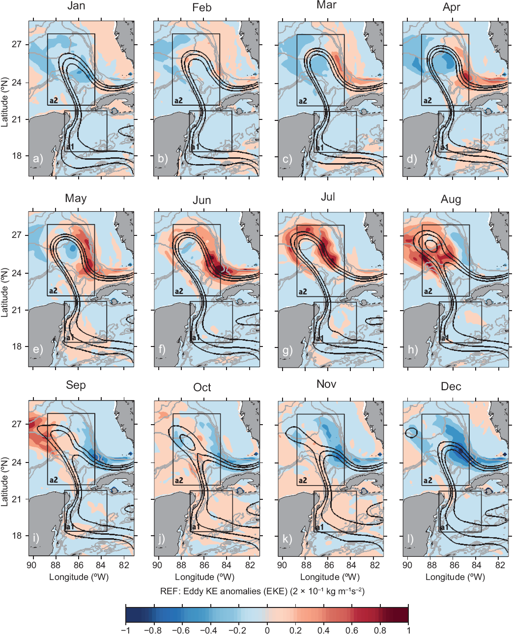
Fig. 11 Monthly mean of the EKE anomaly maps (kg REF: Mean EK anomalies (EKE) [2 x10⁻¹ kg m-1s-2]) of REF experiment averaged in time from 1996-2009 and vertically down to 700 m depth. The solid black lines indicate monthly mean SSH contours of 15, 25, and 35 cm for the same period and mark the LC extension in each experiment. Grey lines show the 500, 1500, and 3000 m isobaths. Boxes a1 and a2 are defined to investigate the mean and eddy flows.
The high EKE region along the northern and eastern rims of the LC is related to LC meanders, LCFEs and enhanced instability energy exchanges in the area (see below). The relative vorticity movie (in the supporting material), shows that a similar -but differently evolving- mechanism is at play in all experiments: cyclonic LCFEs generated on the LC northwestern rim subsequently travel downstream and generate a large LC meander and cyclonic eddy on its eastern side. If the cyclone is strong enough, it can cut the LC anticyclonic bulge and produce or create conditions for an LCE detachment.
The movie shows the evolution of the relative vorticity at 300 m and 1400 m depth. One can see the generation and propagation of LC frontal instabilities on the northeastern rim of the Campeche Bank in the 300 m animations. The relative vorticity at depth (1400 m), has a complicated structure, but clearly depicts the intensification of deep cyclones when they move off the northern slope (Mississippi Fan) towards deep waters near Florida. These cyclones interact with upper layer eddies, become more barotropic, and lead to the LCE separation, a process described in Le Hénaff et al., 2012.
The movie also helps to understand the LC statistics and kinetic energy variability from the experiments. Starting with experiment SMOOTH, we see that the LC, on average, extends less into the GoM, but its mean position presents a high variability. Besides, as long as the LC reaches the Mississippi Fan, the LCFEs can intensify and produce LCE detachment regardless of its lower energy (relative to the other experiments). CANYON has an extended and relatively more stable LC northward position, reaching the northern Campeche Bank more frequently. Except for the very long separation period events (Fig. 7), the statistics suggest it has a more stable LCE separation period. It is difficult to explain why this happens, but we suggest it is related to its relative position with respect to the northern GoM slope and the subtle impact that the absence of the deep canyon has. Intensified cyclones tend to cut the LCE north of the canyon, but when the canyon is presented the cyclones are also intensified there, and this adds a source of variability not evident when the canyon is removed.
Experiments REF and VISCO have a relatively similar distribution of LCE separation events regardless of the lack of Caribbean eddies in the Yucatan area in the latter. It is interesting that VISCO has the largest number of LCE detachments, a fact we suggest is connected to its more extended LC condition to the north and west. If the LC is more extended to the west, intensified cyclones on the western side of the Mississippi Fan can also participate in the LCE detachments. On the other hand, the number of LCE releases is less than in REF. One may think the absence of Caribbean eddies in VISCO might be the cause of this but it is difficult to make the link given the large number of detachments.
In brief, we have seen that the LCE release process is very complicated, and its relation to EKE levels is not as clear as one might expect. It remains to be determined if instability analysis and eddy-mean flow interaction can provide more insight into the problem. This is the subject of the next section, where we investigate the strength and structure of the energy exchange terms associated with instability and their relation to LCE sheddings.
4.4 Barotropic and Baroclinic instability and LCE releases
Instability of the main currents is closely related to the energy evolution and its spatial distribution in the GoM region and may give more clues for explaining the differences among the experiments. To investigate this, we use the energy equations derived by Orlanski and Cox (1972), Beckmann et al. (1994) and Masina et al. (1999). The equations are included in Appendix B for completeness. In what follows, we use the notation of Beckmann et al. (1994). Recall that to focus on perturbations associated to LCFEs, we split the dynamical field into a time-evolving "mean flow" defined using a low-pass filter (cutoff period of 60 days) with the higher frequency fluctuations representing the LCFEs. This required to review that the terms that vanish by definition when the mean flow is defined as the overall time mean, also vanish or are several orders of magnitude smaller than the retained terms in the energy equations. Since we work in an open ocean region, a comprehensive analysis of the energy cycle based on Lorenz (1955) is far harder than in a closed area. The analysis will focus on the energy exchange terms, associated with barotropic and baroclinic instabilities, as found in literature (Orlanski and Cox, 1972; Masina et al.,, 1999; Oey, 2008).
These energy exchange terms are:
 1
1
 2
2
 3
3
 4
4
where u, v, and w are the standard 3d components of the velocity vector; ρ
0 is a constant seawater reference density; g is the acceleration of gravity;
The term T1 represents the transfer of mean (available) potential energy to mean kinetic energy; T2 indicates the transfer of eddy to the mean potential energy; T3 is the transfer of eddy potential energy to eddy kinetic energy; and T4 is a source term of eddy kinetic energy through the work of Reynolds stresses against the mean shear. Positive values of T4 are indicative of barotropic instabilities whereas positive values of T2 and T3 are related to baroclinic instabilities.
Figures 12 and 13 show, respectively, maps of the energy transfer densities (the expressions inside the integrals) of terms T2 and T4 of Eqs. (2) and (4), averaged in time from 1996-2009 and vertically down to 700 m depth for the four experiments.

Fig. 12 Baroclinic transfer rate (kg m-1s-3 from eddy potential energy (EPE) to mean potential energy (MPE) (term T2 in Eq. (2) indicative of baroclinic instability), averaged from 1996-2009 and vertically down to 700 m depth for experiments (a) REF, (b) VISCO, (c) SMOOTH, and (d) CANYON. The solid black lines indicate mean SSH contours of 15, 25, and 35 cm for the same period; grey lines mark the 500, 1500, and 3000 m isobaths.

Fig. 13 Barotropic transfer rate (kg m-1s-3) from MKE to EKE (term T4 in the equation (4) indicative of barotropic instability), averaged over time from 1996-2009 and vertically down to 700 m depth for experiments (a) REF, (b) VISCO, (c) SMOOTH, and (d) CANYON. The solid black lines indicate mean SSH contours of 15, 25, and 35 cm for the same period; grey lines mark the 500, 1500, and 3000 m isobaths.
Looking first at Figure 12, two areas with high positive values of T2 stand out as indicative of baroclinic instability: (1) the eastern side of the LC, between 24-27° N, just south of the Mississippi Fan, which is related to the formation of large meanders of the LC front, that lead to the formation of the cyclonic eddies that produce the LCE detachments in the model; and (2) on the western side of the northeastern tip of the Yucatan peninsula, where isobaths turn abruptly to the west-southwest and seems to be in the region where LCFEs are generated or intensify as discussed before. Negative values (e.g., near the LC exit from the GoM), are indicative of an energy transfer from eddy to mean flow. Maps of the term T3 (not shown) are similar to T2, being particularly strong and positive in the same northeastern LC area. It is worth mentioning that no attempt is made here to extract the divergent part of the eddy heat fluxes of T2 (Marshall and Shutts, 1981), since our study focuses on qualitative characteristics of these terms, particularly their location and strength.
High values of T4, indicative of barotropic instability, are more prominent in the western region and less intense over the eastern area. Negative values, indicating an energy transfer from eddy to mean flow, are now more extended on the eastern side of the LC (Fig. 13).
Experiments REF, VISCO, and CANYON are relatively similar in the structure and amplitude of their energy transfer terms, although there are differences. Notice, for example, that VISCO has larger values of T2 (on the deep region between the Campeche Bank and Mississippi Fan, to the west of the LC, Fig. 12), something we connected to its large number of LCE detachments. Experiment SMOOTH, however, has similar regions of instability but the amplitudes are smaller. Recall experiment SMOOTH produces as many LCE releases as REF (Table II), so the small amplitude of these energy exchange terms does not imply a reduction in the number of LCE releases.
Maps ofthe exchange terms at depths below 1000 m (not shown) display relatively high values in the eastern instability region, slanted towards the deep canyon in experiments REF, VISCO, and SMOOTH. The canyon appears to produce a strengthening of the cyclones from the meandering eastern LC front, when they travel westward. As mentioned above, this may explain why there is a reduced number of LCE releases in experiment CANYON.
The question of whether or not variations in time, strength and position of the instability areas are relevant to the LCE detachment and statistics in a single experiment is addressed in Figure 14, which shows seasonal averages of the T2 density for experiment REF. The strength and geographic characteristics are relatively similar through the seasons, but the number of LCE detachments can be quite different (indicated by the number on the bottom left of each panel). In fact, in other experiments the energy exchange terms may be even slightly weaker in a particular season, but the number of LCE separations can remain high (not shown).

Fig. 14 Seasonal (averaged every three months) of the baroclinic transfer rate (term T2 in Eq. [2]), (kg kg m-1s-3), averaged vertically down to 700 m depth, ([a] winter, [b] spring, [c] summer, and [d] fall) for the period 19962009 for experiment REF. The red number on the Yucatan peninsula indicates the number of LCE detachments (LCE sheddings between brackets) in the season. The solid black lines indicate mean SSH contours of 15, 25, and 35 cm for the same three-month period; grey lines mark the 500, 1500, and 3000 m isobaths. Strength and structure of term T2 are similar throughout the seasons, and there is no clear indication of a relation between LCE shedding and intensified baroclinic mean-eddy flow energy exchange.
The regions of instability in our results coincide with those found by Oey (2008), and the areas of cyclone intensification described by Cherubin et al. (2006) and Le Henaff et al. (2012). Instability processes are definitely linked to the LCE detachment, but the energy analysis indicates that instabilities are ubiquitous in the system, and monthly or seasonal changes in the strength of the instability terms do not provide sufficient guidance to explain differences in the seasonal LCE detachments statistics. Furthermore, the actual LCE separation event is so complicated that high values of the energy exchange terms, indicating enhanced instabilities at a certain time, may not coincide with the actual time when the LCE is released, as we already discussed (section 4.2).
LCE detachments appear to be more connected to the relative position of the LC, which needs to extend sufficiently into the GoM to interact with the northern Campeche Bank, Mississippi Fan, and western Florida slope. The interaction of the LC with these topographic features lead to the final LCE release through a very complicated process that involves the formation and spin-up of LCFEs, the enhancement of vortex instabilities and larger cyclones (Chérubin et al., 2006; Oey, 2008; Le Henaff et al., 2012).
5. Conclusions
The key issue we want to highlight from our numerical sensitivity experiments is that model configurations can bias the LC behavior, and that, in turn, will bias the LCE detachment and separation statistics. The low frequency character of the LCE separation process requires longer time series to obtain robust statistics. However, Kolmogorov-Smirnov tests of the other LC metrics such as northern maximum latitude, from the different experiments, do have significant differences. These biases may not be eliminated even if very long integrations are carried out to obtain more robust LCE shedding statistics. Therefore, a model configuration that, for example, produces a very symmetric distribution in its low and high LC extension (retracted and extended LC modes), is not likely to change even if longer integrations are carried out (Dukhovskoy et al., 2015).
All our experiments reproduce qualitatively key dynamical aspects of the circulation in the GoM but each configuration produces a distinct LC behavior. It is therefore important to consider this situation for model validation and exercise caution when interpreting LCE shedding statistics from a single numerical configuration; several experiments may need to be run in parallel to better understand these statistics.
Several physical mechanisms seem relevant to the LCE shedding process and LC behavior. It seems hard to single out one of them as the most important, but our results suggest that the extension of the LC over the northern slope of the GoM is of primary importance to understand the LCE shedding process. Theories (Pichevin and Nof, 1997; Nof, 2005), based on a reduced gravity one layer model, ignore any role played by the topography, lower layer dynamics and their interaction with upper layer LC. They probably explain the intrusion and growing of the LC bulge into the GoM and its tendency to move westward in more comprehensive models too. Although the Pichevin-Nof mechanism certainly leads to LCE detachments, our results suggest lower layer dynamics and interaction with topography play a primary role, in agreement with Chérubin et al. (2006), Le Henaff et al. (2012) and Hamilton et al. (2015) and not a secondary role as suggested by Xu et al. (2013). The strong relation between transport, LC extension and relative vorticity found in other models (Chang and Oey, 2013) is only present in one of our experiments (SMOOTH) with smooth topography. It is interesting that the models that present that connection also require topography smoothing (Chang and Oey, 2013).
The relative position of the LC with respect to the northern GoM slope and its meridional excursions appear to determine the characteristics of the eddy shedding statistics. That the LC extends sufficiently north to interact with the Mississippi Fan is a necessary, but not sufficient, condition to produce LCE detachments in the model. Instability processes are responsible for LCFEs intensification and LCE detachments, but seasonal variations ofthe source terms (Figs. 12-14) do not provide guidance to explain the seasonal distribution of LCE sheddings. Indeed, the overall dynamics appear extremely complex and in need of further analysis.
Our results highlight the need to take LCE separation statistics produced by models with care given its sensitivity to the model configuration, but they also show their potential to understand essential dynamical features of the GoM numerical models. Given the high and wide spectrum of variability in both models and observations, it seems that the available databases are still not sufficient to clearly define if there are seasonal preferences in the LC shedding statistics. The evidence so far suggests there is, but the mechanisms involved remain uncertain.


