Sensitivity of PBL schemes of the WRF-ARW model in simulating the boundary layer flow parameters for its application to air pollution dispersion modeling over a tropical station

 

Rahul Boadh and A. N. V. Satyanarayana

Centre for Oceans, Rivers, Atmosphere and Land Sciences, Indian Institute of Technology Kharagpur, Kharagpur - 721302, India Corresponding author: A. N. V. Satyanarayana: email: anvsatya@coral.iitkgp.ernet.in

 

T. V. B. P. S. Rama Krishna

Council of Scientific and Industrial Research, National Environmental Engineering Research Institute, Hyderabad - 500007, India

 

Srikanth Madala

Centre for Oceans, Rivers, Atmosphere and Land Sciences, Indian Institute of Technology Kharagpur, Kharagpur - 721302, India

 

Received: March 12, 2015; accepted: November 11, 2015

 

RESUMEN

Las circulaciones atmosféricas de mesoescala desempeñan un papel importante en el transporte de la contaminación del aire y en cuestiones relacionadas con la calidad del aire a nivel local. La estructura termodinámica de la capa limítrofe planetaria (PBL, por sus siglas en inglés) y el campo de flujo también desempeñan un papel importante en la dispersión de contaminantes en la atmósfera. Por lo tanto, se simularon los parámetros de la PBL sobre Naigpur, India, utilizando el modelo de mesoescala ARW v. 3.6.1. Las simulaciones de alta resolución se llevaron a cabo por medio de dominios anidados con resolución horizontal de 27, 9 y 3 km, y 27 niveles verticales obtenidos mediante la utilización de los campos meteorológicos de 1 x 1° del análisis final del NCEP, para las condiciones iniciales y limítrofes. Para estudiar la evolución de los parámetros de la PBL y la estructura termodinámica durante el periodo de estudio, se eligieron ocho días de invierno y verano (enero y abril) con buen tiempo y ausencia de actividad sinóptica significativa. Se realizaron experimentos de sensibilidad del modelo ARW con dos parametrizaciones de la difusión turbulenta del cierre de energía cinética (TKE, por sus siglas en inglés) no locales (Yonsei University [YSU] y el Modelo Convectivo Asimétrico v. 2 [ACM2, por sus siglas en inglés]) y tres locales (Mellor-Yamada-Nakanishi and Niino Level 2.5 PBL [MYNN2], Mellor-Yamada-Janjic [MYJ] y eliminación de escala casi normal [QNSE, por sus siglas en inglés]). La validación de los parámetros simulados mediante el modelo con los datos in situ disponibles reveló que el esquema PBL no local YSU seguido del esquema local MYNN2 podrían reproducir las variables meteorológicas superficiales y la estructura termodinámica de la atmósfera. Los resultados del estudio sugieren que los esquemas PBL, en especial YSU y MYNN2, tuvieron un mejor desempeño para representar los parámetros de la capa limítrofe y son útiles en estudios de dispersión de contaminantes atmosféricos.

 

ABSTRACT

Mesoscale atmospheric circulations play an important role in the transport of air pollution and local air quality issues. The planetary boundary layer (PBL), the thermo-dynamical structure and the flow field play an important role in air pollution dispersion. Hence, the PBL parameters over Nagpur, India are simulated using the ARW v. 3.6.1 mesoscale model. High-resolution simulations are conducted with triple nested domains having a horizontal resolution of 27, 9 and 3 km, as well as 27 vertical levels by using the 1 x 1° NCEP Final Analysis meteorological fields for initial and boundary conditions. Eight fair-weather days in winter and summer (January and April 2009) with no significant synoptic activity were chosen for the study. Sensitivity experiments of the ARW model were conducted with two non-local (Yonsei University [YSU], and Asymmetric Convective Model v. 2 [ACM2]) and three local turbulence kinetic energy (TKE) closure (Mellor-Yamada Nakanishi and Niino Level 2.5 PBL [MYNN2], Mellor-Yamada-Janjic [MYJ], and quasi-normal scale elimination [QNSE]) turbulence diffusion parameterizations, to study the evolution of PBL parameters and the thermodynamical structure during the study period. After validation of the simulated parameters with the available in situ data, it was revealed that the non-local PBL scheme YSU, followed by local scheme MYNN2, could be able to capture the characteristic variations of surface meteorological variables and the thermodynamical structure of the atmosphere. The present results suggest that PBL schemes, namely YSU and MYNN2, performed better in representing the boundary-layer parameters and are useful for air pollution dispersion studies.

Keywords: Planetary boundary layer, WRF, mesoscale, thermodynamical structure.

 

1. Introduction

The planetary boundary layer (PBL) is the lowest 1-3 km region of the atmosphere within the troposphere, characterized by friction and turbulent mixing (Stull, 1988; Garratt, 1994). The boundary-layer processes are especially influential in the evolution of the lower atmospheric flow field and other state parameters. The PBL plays an important role in the transportation of energy (including momentum, heat and moisture) into the upper layers of the atmosphere and acts as a feedback mechanism in wind circulation. The depth and structure of the atmospheric boundary layer are determined by the physical and thermal properties of the underlying surface along with the dynamics and thermodynamics of the lower atmosphere. The thermodynamical state of the PBL plays a significant role in mixing and dispersion of air pollutants.

In particular, the PBL turbulence diffusion plays an important role in the evolution of lower atmospheric phenomena, which in turn determines air pollution dispersion and its transport. PBL parameterization schemes are essential for better simulations of air quality, wind components and turbulence in the lower part of the atmosphere (e.g., Steeneveld et al., 2008; Storm et al., 2009; Hu et al., 2012; García-Diez et al., 2013). The literature indicates that initial as well as boundary conditions, resolution, and physical process parameterizations play an important role in better simulations of atmospheric dynamics (McQueen et al., 1995; Pielke and Uliasz, 1998; Warner et al., 2002; Jiménez et al., 2006).

Though numerical models incorporate well-developed physics such as surface heat, moisture budgets, canopy effects, and boundary-layer turbulent diffusion to resolve the flow, representation of these processes at the model grid resolution is subject to several input data. The thermo-dynamical state ofthe PBL plays important role in mixing and dispersion of air pollutants.

Mesoscale models include complete physics for convection, boundary-layer turbulence, radiation and land-surface processes which play an important role in simulations of various extreme events in general and especially in weather forecasting. The PBL turbulence diffusion in particular plays an important role in the evolution of lower atmospheric phenomena such as convective thunderstorm development, pollution diffusion and transport. PBL parameterization schemes are important for accurate simulations of turbulence, wind and air quality in the lower atmosphere. Some studies were reported in literature regarding the sensitivity of the PBL schemes of mesoscale models (e.g., Srinivas et al., 2007; Li and Pu, 2008; Storm et al., 2009; Miao et al., 2009; Hu et al., 2010, 2012, 2013; López-Espinoza and Zavala-Hidalgo, 2012; García-Diez et al., 2013; Srikanth et al., 2014).

Several recent studies emphasized the role of PBL parameterization in atmospheric simulations with mesoscale models (e.g., Hu et al., 2010; Gilliam and Pleim, 2010; Shin and Hong, 2011; Floors et al., 2013; Yang et al., 2013). Papanatasiou et al. (2010) have used the Weather Research and Forecasting (WRF) modeling system to study the wind field over the east coast of central Greece under summer conditions. Over tropical Indian regions, relatively few studies are available on the performance of PBL schemes in mesoscale models (e.g., Sanjay, 2008; Srinivas et al., 2014, 2015). In a sensitivity experiment of the WRF model for thunderstorm predictions, Srikanth et al. (2014) noticed that the Mellor-Yamada-Janjic (MYJ) local diffusion PBL scheme produced better results over the tropical hilly station Gadanki. Air quality assessment requires accurate predictions of boundary-layer temperature, humidity, winds and mixed-layer depth. The YSU, a non-local diffusion scheme and the MYNN2, a local diffusion scheme captured well the PBL structures over the tropical coastal station Kalpakkam during fair weather conditions (Harip-rasad et al., 2014). Srikanth et al. (2015) studied the sensitivity of different PBL schemes available in the Advanced Research WRF (ARW) mesoscale model in simulating the PBL flow-field and other parameters over Ranchi during different seasons. After validating with available in situ measurements, their study reported that the ACM2 followed by MYNN2 and YSU PBL turbulent diffusion parameterizations has shown better performance in simulating surface meteorological variables. Boadh et al. (2015) have explored the sensitivity of the ARW model over Visakhapatnam and concluded that the non-local schemes YSU followed by ACM2 better simulate surface meteorological variables as well as the ther-modynamical structure of the atmosphere.

In this study the flow-field and atmospheric parameters over the Nagpur region are simulated using ARW v3.6.1 mesoscale model to evaluate its performance for lower atmospheric meteorological fields by conducting sensitivity experiments with various conceptually different PBL schemes.

 

2. Study region

Nagpur (21.15° N, 79.09° E) is the largest city in central India and the second capital of the state of Maharashtra. It is a fast growing metropolis, is the third most populous city in Maharashtra after Mumbai and Pune, and the center for urbanization, development, industrialization and commercial activity. However, the efforts to enhance the green cover of the city, which has a scrubbing effect on air pollutants are scarce. Nagpur has a tropical wet and dry climate (according to the Koppen climate classification) with dry conditions prevailing for most of the year. It is situated 312.42 masl. Summers are extremely hot, lasting from March to June, with May being the hottest month. During the winter period (November to January), temperatures can drop below 10 °C over the region. The highest recorded temperature in the city was 47.9 °C on May 22, 2013, while the lowest was 3.9 °C.

 

3. Data and methodology

3.1 Data and study period

We have used the 1 x 1° final analysis (FNL) data from the National Centre for Environmental Prediction (NCEP) in the present study. For validating the ARW model simulations, available meteorological observations such as wind speed and wind direction at 10 m height, temperature and relative humidity at 2 m height, obtained from the India Meteorological Department (IMD) for Nagpur airport are used. Available upper air radiosonde observations consisting of zonal wind (ms^-1), meridional wind (ms^-1), relative humidity (%) and equivalent potential temperature (K), obtained from the Department of Atmospheric Science, University of Wyoming (http://weather.uywo.edu/upperair/sounding.html), are used for validation of the vertical structure of the atmosphere over Nagpur. Quality control of these data has been conducted as part of the Severe Thunderstorm Observations and Regional Modeling (STORM) program, and quality checks were conducted with DigiCORA radiosondes and found reasonably good (Tyagi et al. , 2013). Additionally, it is noticed from literature (Boadh et al., 2015; Srikanth et al., 2015) and many researchers have used these radiosonde data sets, which ensures the good quality of data and allows us to use it for validation in the present study. Atrri and Tyagi (2010) suggest, according to the IMD, classification of the different seasons as winter (December, January and February), summer or pre-monsoon (March, April and May), monsoon (June, July, August and September) and post-monsoon (October, November). In the present study, to test the model sensitivity of five PBL parameterization schemes, two contrasting months (January, representing the winter season, and April, representing the summer season) are considered. For each month, simulations are conducted for eight fair weather days during which no significant synoptic activities occurred. These days were chosen in order to conduct the performance of the PBL parameterizations without any influence of external weather event influences. Accordingly, in the present study the selected dates for simulations of the WRF model were integrated for a period of 48 h, starting from of 00:00 UTC on January 8-15, 2009 for winter, and 00:00 UTC on April 08-15, 2009 for the summer month, as initial conditions.

3.2 Model description - mesoscale model

To simulate the local scale flow and PBL characteristics over the Nagpur region, the ARW v. 3.6.1, 3-D non-hydrostatic atmospheric mesoscale model is used in the present study. The model consists of an Eulerian mass solver with fully compressible non-hydrostatic equations, terrain following vertical coordinate, and staggered horizontal grid with complete Coriolis and curvature terms. The prognostic variables include three-dimensional wind, perturbation quantities of pressure, geopotential, turbulent kinetic energy surface pressure, potential temperature and scalars (water vapor mixing ratio, cloud water, etc.). A detailed description of the model physics, equations and dynamics is available in Skamarock et al. (2008).

3.3 Model configuration and initialization

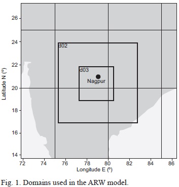
Horizontal and vertical resolution are factors implied in modeling small-scale atmospheric phenomena. Though high resolution results in more precise, better-resolved, small-scale processes, it increases the numerical costs of the model (Mass et al., 2002; Gego et al., 2005; Chou, 201l). For this purpose the WRF model is designed with three nested grids (27, 9 and 3 km) (Fig. 1) and 27 unequally spaced vertical sigma. The outer domain (d01) covers a larger region with a 27 km resolution and 60 x 60 grids. The second inner domain (d02) has a 9 km resolution with 91 x 91 grids, and the innermost domain (d03) has a 3 km resolution with 112 x 112 grids. The second and third nests are two-way interactive domains. The model is run using 1 x 1° six-hourly data from the NCEP FNL for the initial and boundary conditions. The model physics options used are the Kain-Fritsch scheme (Kain, 2004) for convective parameterization, WRF single moment class 6 (WSM6) (Hong et al., 2006) for cloud microphysics, the NOAH land surface model (Chen and Dudhia, 2001) for surface physics, the Rapid Radiative Transfer Model (Mlawer et al., 1997) for long-wave radiation processes, and the Dudhia scheme for short wave radiation (Dudhia, 1989). The modeling domains and configuration are presented in Table I.

3.4 PBL sensitivity experiments

The PBL parameterizations and land surface influence the simulation of turbulence, winds, and other state variables in the lower atmosphere. In the present study, to test the model sensitivity five PBL parameterizations schemes, namely two non-local schemes (Yonsei University [YSU] [Hong et al., 2006], and Asymmetric Convective Model v. 2 [ACM2] [Pleim, 2007]), and three local turbulence kinetic energy (TKE) closure (Mellor-Yamada Nakanishi and Nii-no Level 2.5 PBL [MYNN2] [Nakanishi and Niino, 2004], Mellor-Yamada-Janjic [MYJ] [Janjic, 2002], and quasi-normal scale elimination [QNSE] [Suko-riansky et al., 2005]) are selected. Several recent studies emphasize the role of PBL parameterization in atmospheric flow-field simulations (e.g., Skamarock et al., 2008; Shin and Hong, 2011; Xie et al., 2012; Floors et al., 2013; Srikanth et al., 2014; Hariprasad et al., 2014; Kleczek et al., 2014, Boadh et al., 2015; Srikanth et al. , 2015).

3.5 Model validation and statistical evaluation

The model-generated surface meteorological variables such as air temperature (AT), relative humidity (RH) at 2 m, wind speed (WS), wind direction (WD) 10 m above the ground level, and vertical profiles of zonal wind, meridional wind, relative humidity and equivalent potential temperature during the study period (representative days of the summer and winter seasons) are validated with the available surface meteorological observations as well as radiosonde observations. Results are compared qualitatively and quantitatively for both surface meteorological variables as well as the thermodynamical structure of the atmosphere. Quantitative comparisons are based on error statistics mean bias (MB), mean absolute error (MAE), root mean square error (RMSE) and correlation coefficient (CC) (Wilks, 2011).

 

4. Results and discussion

4.1 Surface meteorological parameters

In this section an intercomparison of performance of various PBL parameterization schemes in simulating the diurnal variation of surface meteorological variables such as AT (°C), RH (%), WS (ms^-1) and WD (°), along with in situ observations at hourly intervals at the Nagpur station, is presented.

4.1.1 Air temperature

The diurnal variation of air temperature (AT) in January 2009 is shown in Fig. 2. The model was able to capture a similar trend of evolution for the diurnal variation as seen in the observations. During nighttime, a slight cold mean bias (i.e., observation-model < 0) is noted in January 2009. The MYJ, MYNN2 and YSU are closer to the observations in comparison with the rest of the schemes. Based on the analysis, more cold bias has been noticed with the simulations using the QNSE scheme than with the other schemes during nighttime. During daytime, all PBL schemes are in good agreement with the observation. The diurnal variation of AT in April 2009 has been depicted in Fig. 3, and it can be noticed that all PBL schemes exhibits cold mean bias. In general comparison, one can see that, YSU, MYJ and MYNN2 schemes are in good agreement with the observations in comparison with the other scheme. Overall, QNSE simulations of AT have shown more cold bias during nighttime both during January and April, whereas all the PBL schemes are in agreement with the observations. Similar results are reported by García-Diez et al. (2013) over Europe and Srikanth et al. (2015) over Ranchi. On close examination, it is noticed that non-local scheme YSU and local schemes MYNN2 and MYJ simulate AT reasonably well.

4.1.2 Relative humidity (RH)

The diurnal variation of relative humidity (RH) during January and April 2009 is shown in Figs. 4 and 5, respectively, over Nagpur. RH is overestimated by most of the schemes, but they were able to capture the similar trend of diurnal variation, as shown in the observations during both months. It is clearly seen in Fig. 5 that RH is lower in April because Nagpur is hot and dry during summer.

In general, YSU, ACM2 and MYJ schemes better simulated the RH and captured the diurnal variation reasonably well as compared to other schemes. In January and April, the local scheme QNSE simulated a higher magnitude of RH compared to other schemes. The overestimation of RH by QNSE may be attributed to cold bias. Similar type of the variations has been reported by Srikanth et al. (2015) over Ranchi and Hariprasad et al. (2014) over Kalpakkam.

4.1.3 Wind speed and direction Comparisons of wind speed (WS) and direction (WD) are made through joint frequency distribution plots and henceforth referred to as wind roses. The wind roses of model-generated WS and WD are compared with observations for all study days during both January and April 2009. In the present study, wind roses are prepared together for the eight chosen days during January and April; they are compared with observations in Figs. 6 and 7, respectively.

Observed wind roses during January 2009 (Fig. 6f) reveal that winds blow mostly from the east, northeast and southeast. MYNN2 (Fig. 6b) and YSU (Fig. 6a) show similar patterns but with smaller magnitudes. Regarding wind direction, MYNN2, YSU, and ACM2 (Fig. 6e) produced smaller magnitudes but were able to capture the easterly and northeasterly winds.

In January, MYJ and QNSE produced high wind speeds (4-6 ms^-1) compared to other PBL schemes (YSU, MYNN2 and ACM2) in the east and east-southeast directions. The wind roses for April (Fig. 7) show strong wind speeds (6-8 ms^-1) from north and north-northeast winds and moderate north-northwest winds simulated by the ACM2, QNSE and MYJ schemes (Fig. 7e, d, c). Winds from north and north-northwest directions simulated by the YSU and MYNN2 schemes (Fig. 7a, b, respectively) with moderate wind speeds (4-6 ms^-1) followed slightly similar patterns of observation, but with different magnitude.

Overestimation of winds seems to be a common experience with the WRF model, which was also reported by earlier works (e.g., Srikanth et al., 2013; Zhang et al., 2013; Hariprasad et al., 2014; Srikanth et al., 2015). In general, during both January and April, model simulated winds by the non-local YSU and ACM2 schemes, and the local MYNN2 scheme were better able to capture low wind conditions as compared to MYJ and QNSE, as can be seen in the observations. The overestimation of winds by the WRF may be attributed to the non-accurate prescription of surface roughness and induced turbulence intensity in the atmospheric surface layer.

Hariprasad et al. (2014) have shown that YSU and MYNN2 produce better PBL structures over the tropical coastal station Kalpakkam during fair weather conditions. Srikanth et al. (2015) have also shown that YSU, MYNN2 and ACM2 produce better PBL structures over Ranchi. In general, our results support and confirm that the YSU, MYNN2 and MYJ schemes produce better PBL structures over the Nagpur region. Based on qualitative comparisons, we noticed that YSU followed by MYNN2 simulated most surface meteorological parameters reasonably well in both January and April as compared to the other tested PBL schemes.

4.2 Thermodynamical structure of the atmosphere

In this section we discuss the vertical profiles of zonal winds (ms^-1), meridional wind (ms^-1), relative humidity (%) and equivalent potential temperature (K) derived from simulations using different PBL schemes along with available radiosonde observations. In Figure 8, the purpose of using 6_e instead of potential temperature (6) is that the former is a conserved variable and better represents convective instability (Tyagi et al., 2013). Radiosonde observations data were obtained from the Department of Atmospheric Science, University of Wyoming. Since these radiosonde observations are only available at 00:00 UTC (05:30 LT), model simulations are only validated during this time. This is one of the limitations of the present study.

For the sake of continuity, we show the results for two days (January 10 and 13, 2009) for the winter month (Fig. 8) and two days (April 11 and 13, 2009) for the summer month (Fig. 9). Model simulated profiles for zonal wind (ms^-1) (a, e), meridional wind (ms^-1) (b, f), relative humidity (%) (c, g), and equivalent potential temperature 6_e (K) (d, h), as well as parameters derived from radiosonde observations over Nagpur at 05:30 LT on January 10 and 13, 2009, and April 11 and 13, 2009, are shown in Figures 8 and 9, respectively. In general, and mostly for the winter month, winds in the lower atmosphere up to 200 m (which can be seen in the observed profiles of zonal and meridional winds in Fig. 8a, b, e, f), blow in the northeast direction. The change of wind direction to the southeast in the 200-1500 m layer, and subsequently to the southwest in the 1500-2200 m layer and to the northwest above this height, can be noticed in the radiosonde observations.

For summer, winds in the lower atmosphere are mostly northerly, and up to 600 m they are northeasterly; above that, most winds are found to be westerly and northwesterly, which can be noticed in the radiosonde observations (Fig. 9a, b, e, f). All the PBL schemes reasonably simulated vertical variations of wind speed and direction for both seasons. For winter, RH in the lower atmosphere up to 3000 m was around 50-80% (Fig. 8c, g), and for summer a smaller magnitude of RH around 15-30% was noticed in observations (Fig. 9c, g). RH variation for January and April was well simulated in all the PBL schemes. Equivalent potential temperature in morning profiles generally shows stable conditions with stable layers -500 m during the winter month and ~300 m over the summer month. The observed vertical variation of equivalent potential temperature was well captured by all PBL schemes except for a smaller magnitude (around 2-3 K) for the lower atmosphere up to 500 m over the winter month (Fig. 8d, h) and a higher magnitude around 2 K for the summer month (Fig. 9d, 9h).

The analysis of vertical profiles of the above parameters reveals a clear-cut variation both in January and April. These characteristics are well simulated by all PBL schemes, though with few differences. Based on the results it can be observed that qualitatively the YSU followed by the MYNN2 scheme has reasonably simulated the PBL vertical thermodynamical structure of the atmosphere as compared to other PBL schemes over the Nagpur region.

4.3 Statistical analysis of surface meteorological variables and the thermodynamical structure of the atmosphere

A statistical analysis based on MB, MAE, RMSE and CC between simulated and observed surface meteorological variables such as AT, RH, WS and WD with five PBL schemes for the simulation period (eight days in January 2009 and 8 days in April 2009) are given in Table II. Since the direct comparison of simulated and observed wind directions can lead to large errors whenever wind fluctuations occur around 0°/360°, wind direction errors are assessed by comparing the vector winds (u, v) (Srikanth et al., 2015). It has been found that all the PBL schemes simulated a cold bias in temperature with YSU and MYJ, giving lesser errors and higher correlations compared to other PBL schemes. For RH, all PBL schemes produced a humid bias. The relatively lesser errors and good correlations obtained with YSU and ACM2 indicate these schemes simulate the RH better than other PBL schemes. The error statistics for winds show that a slight overestimation of their strength is noticed in the MYJ, QNSE, and YSU schemes. However, the smaller RMSE and higher correlations obtained from YSU, ACM2 and MYNN2 indicate these schemes have simulated wind speed reasonably well. Although most schemes adequately simulated wind direction, the higher correlations and lesser errors obtained with YSU, MYNN2 and ACM2 confirm that these schemes simulated better the wind direction than the other two schemes.

Overall, for various surface meteorological variables, the YSU and MYNN2 schemes produced lesser errors and were in better agreement with observations within the study region. A statistical analysis of MB, MAE, RMSE and CC between simulated and observed vertical profiles of zonal and meridional wind components, relative humidity and equivalent potential temperature using five PBL schemes along with available observations, are given in Table III. Mean statistics show that all PBL schemes produce a cold bias in RH and a cold mean bias (i.e., model-observation < 0) in equivalent potential temperature.

Overall, regarding surface meteorological variables as well as the thermodynamical structure of the atmosphere, the YSU and MYNN2 schemes produced lesser errors and were in better agreement with observations within the study region compared to other PBL schemes.

4.4 Sensible heat flux, latent heat flux and momentum flux

Surface fluxes such as sensible heat (Q_H), latent heat (Q_E) and momentum flux (MF) transported from the atmospheric surface layer to the atmosphere above play a vital role in defining the vertical profiles of temperature, humidity and wind components in the atmospheric boundary layer. In the present study, the diurnal variation of these fluxes simulated with different PBL schemes of the WRF model are presented in Figures 10 and 11, for January 10 and 13, 2009, and April 11 and 13, 2009, respectively.

Though all the PBL schemes simulated nearly similar values of nighttime Q_H, significant differences are found in daytime fluxes, especially in afternoon hours (Fig. 10a, b and Fig. 11a, b) during both January and April. The daily cycle shows in general higher fluxes in model simulated Q_H with QNSE and MYJ, compared to other schemes. Higher heat flux would lead to a strongly convective atmosphere and growth of deep daytime PBLs (Srikanth et al., 2015). It is also noticed that QH magnitudes are higher during April than in January.

The diurnal variation of latent heat flux (Q_E) is shown in Figure 10c, d, and Figure 11c, d) during January and April. As seen in the QH diurnal variation, a similar trend is noticed in QE. In general, QNSE, MYJ simulated higher magnitudes of QE compared to the other schemes.

A higher momentum flux (MF) was noticed during April compared to that of January as shown in Fig. 10e, f, and Fig. 11e, f). As with Q_H and Q_E, the WRF model with QNSE and MYJ simulated a higher MF during April. From the analysis, it is noticed that PBL schemes differ in the simulation of these fluxes during both January and April. From these case studies, it was observed that YSU and MYNN2 simulated smaller magnitudes of these fluxes compared to QNSE, MYJ and ACM2.

4.5 PBL height, convective velocity scale and ventilation coefficient

Here we discuss the PBL height (PBLH) (also called mixed layer height), which attains significance in air quality dispersion assessment, the convective velocity scale (W*), also called mixing scaling parameter, and the ventilation coefficient (VC). The VC is the product of the average wind speed and mixing layer height, which means that VC shows the capacity of the atmosphere to disperse and reduce the pollutants over a region. VC is used as a direct measure to differentiate the degree of transport/dispersion of pollutants taking place within the con-vective boundary layer. It reflects the transport rate of populations in the mixing layer. Higher values of VC indicate effective dispersion. The calculation of VC is given by

where X_i is the atmospheric mixing layer height above the ground (m), and Y is the wind speed near the ground (ms^-1). Viswanahdam et al. (1993, 1995, 1997) reported the climatological atmospheric dilution indices, the dispersive capacity of the atmosphere, and the utility of surface meteorological variables in atmospheric dispersion studies over Indian cities.

PBLH predictions are important for the estimation of mean quantities (temperature, wind, etc.) in meteorological models, and are also important for air pollutant dispersion modeling (Carruthers et al., 1994; Cimorelli et al., 2005; Steeneveld et al., 2008; Garcia Diez et al., 2013; Boadh et al., 2015). It represents the effective region of turbulent mixing for heat, moisture and pollutants. Errors in simulating the mixed-layer depth would affect the mixing of pollutants. Deep mixed layers enhance the dispersion while shallow layers restrict the vertical diffusion of pollutants. The employed PBL schemes in the present study estimate the PBLH differently. Hence, in our study we used the model derived vertical profiles of wind components and temperature, and we estimated the PBLH based on the approach suggested by Voge-lezang and Holtslag (1996). We computed the PBLH with all five schemes for stable, unstable and neutral conditions. Simulations were made for PBLH, W* and VC for all eight days both in January and April. For the sake of continuity we show the analysis for January 10 and 13, 2009, and April 11 and 13, 2009 in Figures 12 and 13, respectively.

The diurnal variation of PBLH obtained using various PBL schemes over Nagpur on January 10 and 13, 2009 is shown in Fig. 12a, b respectively, and during summer on April 11 and 13, 2009 in Fig. 13a, b. We could not make direct comparisons of the simulated PBLH against observations, since observed PBLH measurements are not available. However, an intercomparison of values from different numerical experiments provides the relative performance of different PBL schemes.

The PBL schemes YSU and MYNN2 produce shallow boundary layers in January and April, while ACM2 and MYJ produce moderate deep boundary layers in both months. In general, it is noticed that YSU and MYNN2 simulated relatively shallow boundary layers (PBLH ~1600 ± 300 m); ACM2 and MYJ produced moderate boundary layers (PBLH ~2300 ± 300 m), and QNSE produced deeper layers (PBLH ~2900 ± 200 m) during January. For April, YSU and MYNN2 also simulated relatively shallow boundary layers (PBLH ~2300 ± 200 m), ACM2 and MYJ moderate boundary layers (PBLH ~2700 ± 400 m) and QNSE deeper layers (PBLH ~4500 ± 250 m). The diurnal cycle of simulated PBL heights indicates the QNSE produces relatively deep boundary layers in both January and April. QNSE yielded deep boundary layers because it produced significantly high sensible heat flux compared to other PBL schemes. Kompalli et. al. (2014) found the deeper mixing height during summer (~3014 ± 1187 m) and the shallower mixing height during winter (~1488 ± 706 m) over Nagpur. Deep boundary layers with QNSE, ACM2 were also reported by Hariprasasd et al. (2014) at a tropical coastal site (Kalpakkam); Shin and Hong (2011) at mid-latitudes, and Srikanth et al. (2015) over Ranchi. The mixing extremes with the QNSE and ACM2 schemes found in our study support the results of earlier simulation studies.

The convective velocity scale is also called mixing scaling parameter. Venkatram (1978) compared his theory to estimate different W* values at different PBLHs with boundary layer data obtained during the 1973 Minnesota experiment (Kaimal et al., 1976). The diurnal variation of W* during daytime convection (W* > 0) obtained using various PBL schemes on January 10 and 13, 2009 is shown in Fig. 12c, d, respectively, while for April 11 and 13, 2009 it is shown in Fig. 13c, d. In January, all PBL schemes except QNSE simulated smaller magnitudes of W*, as seen in Fig. 12c, d. It can be noticed that QNSE simulated higher values (~2.5 ms^-1), whereas values simulated by MYNN2 were smaller (~1.7 ms^-1), and simulations by other schemes were within this range of magnitude. W* is higher in April, as shown in Fig. 13c, 3d as compared to January. Among the PBL schemes, QNSE simulated higher values (~3.9 ms^-1), and MYNN2 smaller values (~2.7 ms^-1). The higher W* during April is attributed to a more convective uplift due to sensible heat flux compared to that of January over the study region.

The variation in VC during daytime and nighttime on January 10 and 13, and April 11 and 13, 2009 is shown in Figures 12e, f, and 13e, f, respectively. The VC tended to be higher and significantly varied during daytime, while it was relatively lower and constant during nighttime in both months. Similar results were reported by Goyal and Chalapati (2007) for Kochi, who stated that VC was higher during the afternoon while it was lower during the evening and morning in all seasons. QNSE produces a higher VC (~8 x 10³ m² s^-1 during winter and ~195 x 10³ m² s^-1 in the summer), while MYNN2 and MYJ produce a lower VC (~2 x 10³ m² s^-1 in January and ~8.5 x 10³ m² s^-1 in April, respectively) compared to other schemes.

Kompalli et. al. (2014) estimated the VC and found its minimum mean value (~5.7 x 10³ ± 0.4 x 10³ m² s^-1) in January and its maximum (~15.160 x 10³ m² s^-1) in April 2012. We found results within the range for VC in January 2009 on different days: ~5 x 10³ ± 0.5 x 10³ m² s^-1; however, in April it was underestimated: ~8 x 10³ ± 0.4 x 10³ m² s^-1. It was found that VC was extensively variable and high during daytime, while it was quite invariable and low during nighttime, showing a higher dispersion capacity of the PBL during daytime and lower during nighttime.

 

5. Summary and conclusions

The main aim of the present study is to evaluate the performance of various PBL schemes of the WRF-ARW model in simulating the characteristics of me-soscale meteorological parameters over Nagpur for the application of air pollution dispersion studies. The model is integrated with high resolution (3 km) to capture the boundary layer flow parameters over different topographical fluctuations over the study region. Simulations were performed for winter and summer in order to study the application of simulated meteorology in air quality assessment. Sensitivity experiments were conducted using two non-local (YSU, ACM2) and three local (MYNN2, MYJ, QNSE) turbulence kinetic energy (TKE) closure PBL turbulent diffusion parameterization schemes. The simulated thermodynamical structure of the atmosphere and surface meteorological variables were validated with available observations over the study region. Results indicate that the model could capture the local scale flow field and site-specific meteorological variables at Nagpur. Simulations show widely varying flows, mixed layer height, and air temperature both in January and April that would impact the plume trajectory from pollutant sources around the Nagpur region. The analysis of different meteorological variables shows that these are sensitive to the PBL parameterization employed in the model. In general, it has been found that for most variables, non-local scheme YSU and the level 2.5 TKE scheme MYNN2 were in better agreement with observations, both qualitatively and quantitatively. The model simulated deep to very deep boundary layers during summer and shallow layers during winter. Among the different PBL parameterization schemes, QNSE followed by ACM2 and MYJ simulated relatively deep boundary layers, and MYNN2 and YSU simulated relatively shallow layers in both months (January and April). The VC simulated by QNSE compared to other schemes in both months (January and April). In January, VC values simulated by all PBL schemes were much lower than observations, which means pollution values may be very high in Nagpur during January. A lower VC was simulated with YSU followed by MYNN2 during the study periods. A statistical analysis based on MB, MAE, RMSE and CC revealed that YSU and MYNN2 scheme produced smaller errors and were in better agreement with observations regarding surface meteorological variables and the thermodynamical structure of the atmosphere over the study region, compared to other PBL schemes. Within its limitations, the study advocates that non-local scheme YSU followed by local TKE scheme MYNN2 are suitable for air pollution dispersion modeling studies over Nagpur.

 

Acknowledgments

Rahul Boadh would like thank the Indian Institute of Technology Kharagpur for providing research fellowship and necessary facilities to conduct his Ph.D. work. The first author gratefully acknowledges Dr. S. R. Wate, Director of NEERI, Nagpur for giving the necessary permissions and providing facilities to carry out part of the research in NEERI Nagpur. Authors are grateful with two anonymous reviewers for their suggestions and comments for improving the quality of the manuscript.

 

References

Attn S. D. and A. Tyagi, 2010. Climate profile of India. Met Monograph No. Environment Meteorology-01/2010. Environment Monitoring and Research Centre, India Meteorological Department, New Delhi, 122 pp.         [ Links ]

Boadh R., A. N. V. Satyanarayana, T. V. B. P. S. Rama Krishna and S. Madala, 2015. Sensitivity of PBL parameterization schemes of weather research forecasting model and integration with AERMOD in the dispersion of NO_X over a coastal region of southern Visakhapatnam (India). Asia-Pac. J. Chem. Eng. 10, 356-368.         [ Links ]

Carruthers D. J., R. J. Holroyd, R. J. Hunt and J. C. R. Weng, 1994. UKADMS: A new approach to modelling dispersion in the Earth's atmospheric boundary-layer. J. Wind Eng. Ind. Aerodyn. 52, 139-153.         [ Links ]

Chen F. and J. Dudhia, 2001. Coupling an advanced land-surface/ hydrology model with the Penn State/ NCAR MM5 modeling system. Part I: Model description and implementation. Mon. Weather Rev. 129, 569-585.         [ Links ]

Chou S. H., 2011. An example of vertical resolution impact on WRF-Var analysis. Electron. J. Oper. Meteorol. 12, 1-20.         [ Links ]

Cimorelli A. J., S. G. Perry, A. Venkatram, J. C. Weill, R. J. Paine, R. B. Wilson, R. F. Lee, W. D. Peters and R. W. Brode, 2005. AERMOD: A dispersion model for industrial source applications. Part I: General model formulation and boundary-layer characterization. J. Appl. Meteorol. 44, 682-693.         [ Links ]

Dudhia J., 1989. Numerical study of convection observed during the winter monsoon experiment using a me-soscale two-dimensional model. J. Atmos. Sci. 46, 3077-3107.         [ Links ]

Floors R., C. L. Vincent, S. E. Gryning, A. Peña and E. Batchvarova, 2013. The wind profile in the coastal boundary layer: Wind lidar measurements and numerical modelling. Bound.-Lay. Meteorol. 147, 469-491.         [ Links ]

García Diez M., J. Fernández, L. Fitaand C. Yague, 2013. Seasonal dependence of WRF model biases and sensitivity to PBL schemes over Europe. Q. J. R. Meteorol. Soc. 139, 501-514.         [ Links ]

Garratt J. R., 1994. The atmospheric boundary layer. Cambridge University Press, 316 pp (Cambridge Atmospheric and Space Science Series).         [ Links ]

Gego E., C. Hogrefe, G. Kallos, A. Voudouri, J. Irwin and S. Rao, 2005. Examination of model predictions at different horizontal grid resolutions. Environ. Fluid Mech. 5, 63-85.         [ Links ]

Gilliam R. C. and J. E. Pleim, 2010. Performance assessment of new land surface and planetary boundary layer physics in the WRF-ARW. J. Appl. Meteorol. Climatol. 49, 760-774.         [ Links ]

Goyal S. K. and R. C. V. Chalapati, 2009. Assessment of atmospheric assimilation potential for industrial development in an urban environment: Kochi (India). Sci. Total Environ. 376, 27-39.         [ Links ]

Hariprasad K. B. R. R., C. V Srinivas, A. Bagavath Singh, S. Vijaya Bhaskara Rao, R. Baskaran and B. Venkatra-man, 2014. Numerical simulation and intercomparison of boundary layer structure with different PBL schemes in WRF using experimental observations at a tropical site. Atmos. Res. 145, 27-44.         [ Links ]

Hong S. Y. and J. J. O. Lim, 2006. The WRF single-moment microphysics scheme (WSM6). J. Korean Meteor. Soc. 42, 129-151.         [ Links ]

Hu X.-M., J. W. Nielsen-Gammon and F. Zhang, 2010. Evaluation of three planetary boundary layer schemes in the WRF model. J. Appl. Meteorol. Climatol. 49, 1831-1844.         [ Links ]

Hu X.-M., D. C. Doughty, K. J. Sanchez, E. Joseph and J. D. Fuentes, 2012. Ozone variability in the atmospheric boundary layer in Maryland and its implications for vertical transport model. Atmos. Environ. 46, 354-364.         [ Links ]

Hu X.-M., P. M. Klein and M. Xue, 2013. Evaluation of the updated YSU planetary boundary layer scheme with in WRF for wind resource and air quality assessments. J. Geophys. Res. Atmos. 118, 10490-10505.         [ Links ]

Janjic Z. I., 2002. Nonsingular implementation of the Mellor-Yamada level 2. 5 scheme in the NCEP meso model. NCEP Office Note. No. 437. National Centers for Environmental Prediction, 61 pp.         [ Links ]

Jiménez P., O. Jorba, R. Parra and J. M. Baldasano, 2006. Evaluation of MM5-EMICAT2000-CMAQ performance and sensitivity in complex terrain: High-resolution application to the north-eastern Iberian Peninsula. Atmos. Environ. 40, 5056-5072.         [ Links ]

Kaimal J. C., J. C. Wyngaard, D. A., Haugen, O. R. Cote, Y. Izumi, S. J. Caughey and C. J. Readings, 1976. Turbulence stucture in convective boundry layer. J. Atmos. Sci. 22, 2152-2169.         [ Links ]

Kain J. S., 2004. The Kain-Fritsch convective parameterization: An update. J. Appl. Meteorol. 43, 170-181.         [ Links ]

Kleczek M. A., G. J. Steeneveld and A. A. M. Holtslag, 2014. Evaluation of the weather research and forecasting mesoscale model for GABLS3: impact of boundary-layer schemes, boundary conditions and spin-up. Bound.-Lay. Meteorol, doi:10.1007/s10546-014-9925-3.

Kompalli S. K., S. S. Babu, K. K. Moorthy, M. R. Manoj, N. V. P. Kiran Kumar, K. H. F. B. Shaeb and A.. K. Joshi, 2014. Aerosol black carbon characteristics over Central India: Temporal variation and its dependence on mixed layer height. Atmos. Res. 147-148, 27-37.         [ Links ]

Li X. and Z. Pu, 2008. Sensitivity of numerical simulation of early rapid intensification of Hurricane Emily (2005) to cloud microphysical and planetary boundary layer parameterizations. Mon. Weather Rev. 136, 4819-4838.         [ Links ]

López-Espinoza E. D. and J. Zavala-Hidalgo, 2012. Weather forecast sensitivity to changes in urban land covers using the WRF model for central Mexico. Atmósfera 25, 127-154.         [ Links ]

Mass C. F., D. Ovens, K. Westrick and B. A. Colle, 2002. Does increasing horizontal resolution produce more skillful forecasts. Bull. Am. Meteorol. Soc. 83, 407-430.         [ Links ]

McQueen J. T., R. R. Draxler and G. D. Rolph, 1995. Influence of grid size and terrain resolution on wind field predictions from an operational mesoscale model. J. Appl. Meteorol. 34, 2166-2181.         [ Links ]

Miao J. F., K. Wyser, D. Chen and H. Ritchie, 2009. Impacts of boundary layer turbulence and land surface process parameterizations on simulated sea breeze characteristics. Ann. Geophys. 27, 2303-2320.         [ Links ]

Mlawer E. J., S. J. Taubman, P. D., Brown, M. J. Iacono and S. A. Clough, 1997. Radiative transfer for inho-mogeneous atmosphere: RRTM, a validated correlated-k model for the longwave. J. Geophys. Res. 102, 16663-16682.         [ Links ]

Nakanishi M. and H.Niino, 2004. An improved Mellor-Yamada level-3 model with condensation physics: Its design and verification. Bound-Lay. Meteorol. 112, 1-31.         [ Links ]

Pielke R. A. and M. Uliasz, 1998. Use of meteorological models as input to regional and mesoscale air quality models limitations and strengths. Atmos. Environ. 32, 1455-1466.         [ Links ]

Pleim J. E., 2007. A combined local and nonlocal closure model for the atmospheric boundary layer, Part I model description and testing. J. Appl. Meteorol. Climatol. 46, 1383-1395.         [ Links ]

Sanjay J., 2008. Assessment of atmospheric boundary-layer processes represented in the numerical model MM5 for a clear sky day using LASPEX observations. Bound-Lay. Meteorol. 129, 159-177.         [ Links ]

Shin H. H. and S. Y. Hong, 2011. Intercomparison of planetary boundary-layer parameterizations in the WRF model for a single day from CASES-99. Bound.-Lay. Meteorol. 139, 261-281.         [ Links ]

Skamarock W. C., J. B. Klemp, J. Dudhia, D. O. Gill, D. M. Barker, M. G. Dudha, X. Huang, W. Wang and Y. Powers, 2008. A description of the advanced research WRF Ver.30. NCAR Technical Note. NCAR/TN-475+STR. National Centre for Atmospheric Research, Boulder, CO, 113 pp.         [ Links ]

Srikanth M., A. N. V. Satyanarayana and B. Tyagi, 2013. Performance evaluation of convective parameterization schemes of WRF-ARW model in the simulation of pre-monsoon thunderstorm events over Kharagpur using STORM data sets. Int. J. Comput. Appl. 71, 43-50.         [ Links ]

Srikanth M., A. N. V. Satyanarayana and T. N. Rao, 2014. Performance evaluation of PBL and cumulus parameterization schemes of WRF ARW model in simulating severe thunderstorm events over Gadanki MST radar facility - Case study. Atmos. Res. 139, 1-17.         [ Links ]

Srikanth M., A. N. V. Satyanarayana, C. V. Srinivas and M. Kumar, 2015. Mesoscale atmospheric flow-field simulations for air quality modelling over complex terrain region of Ranchi in eastern India using WRF. Atmos. Environ. 107, 315-328.         [ Links ]

Srinivas C. V., R. Venkatesan and A. Bagavath Singh, 2007. Sensitivity of mesoscale simulations of land-sea breeze to boundary layer turbulence parameterization. Atmos. Environ. 41, 2534-2548.         [ Links ]

Srinivas C. V., P. T. Rakesh, K. B. R. R. Hariprasad, R. Venkatesan, R. Baskaran and B. Venkatraman, 2014. Assessment of atmospheric dispersion and radiological impact from the Fukushima accident in a 40-km range using a simulation approach. Air Quality, Atmosphere & Health 7, 209-227.         [ Links ]

Srinivas C. V., K. B. R. R. Hariprasad, C. V. Naidu, R. Baskaran and B. Venkatraman, 2015. Sensitivity analysis of atmospheric dispersion simulations by FLEXPART to the WRF simulated meteorological predictions in a coastal environment. Pure Appl. Geophys., doi:10.1007/s00024-015-1104-z.

Steeneveld G. J., T. Mauritsen, E. I. F. DeBruijn, J. V G. De Arellano, G. Svensson and A. A. M. Holtslag, 2008. Evaluation of limited-area models for the representation of the diurnal cycle and contrasting nights in CASES-99. J. Appl. Meteorol. Climatol. 47, 869-887.         [ Links ]

Storm B., J. Dudhia, S. Basu, A. Swift and I. Giammanco, 2009. Evaluation of the Weather Research and Forecasting model on forecasting low-level jets: Implications for wind energy. Wind Energy 12, 81-90.         [ Links ]

Stull R. B., 1988. An introduction to boundary layer meteorology. Kluwer Academic Publishers, Dordrecht, Boston, London, 666 pp.         [ Links ]

Sukoriansky S., B. Galperin and V. Perov, 2005. Application of a new spectral theory of stably stratified turbulence to the atmospheric boundary layer over sea ice. Bound.-Lay. Meteorol. 117, 231-257.         [ Links ]

Tyagi B., A. N. V Satyanarayana and N.K. Vissa, 2013. Thermodynamical structure of atmosphere during pre-monsoon thunderstorm season over Kharagpur as revealed by STORM data. Pure Appl. Geophys. 170, 675-687.         [ Links ]

Venkatram A., 1978. Estimating the convective velocity scale for diffusion applications. Bound.-Lay. Meteorol. 15, 447-452.         [ Links ]

Viswanadham D. V., A.N.V. Satyanarayana and L. Prasad, 1993. Some aspects of surface layer for direct use in air pollution. Indian Journal of Environmental Protection 13, 179-184.         [ Links ]

Viswanadham D.V., A.N.V. Satyanarayana and Stuti Mishra, 1995. Climatological atmospheric dilution indices over India. Indian Journal of Environmental Protection 15, 734-738.         [ Links ]

Viswanadham D.V., Stuti Mishra and A.N.V. Satyanaraya-na, 1997. Concept and assessment of dilution hours over India. Indian Journal of Environmental Protection, 296-299.

Vogelezang D. H. P. and A. A. M. Holtslag, 1996. Evaluation and model impacts of alternative boundary-layer height formulations. Bound.-Lay. Meteorol. 81, 245-269.         [ Links ]

Warner, T. R., R. S. Sheu, J. F. Bowers, R. I. Sykes, G.C. Dodd and D. S. Henn, 2002. Ensemble simulations with coupled atmospheric dynamic and dispersion models: Illustrating uncertainties in dosage simulations. J. Appl. Meteorol. 41, 488-504.         [ Links ]

Wilks, D. S., 2011. Statistical methods in the atmospheric science, 3rd ed. Elsevier Academic Press, 704 pp.         [ Links ]

Xie B., J. C. H. Fung, A. Chan and A. Lau, 2012. Evaluation of nonlocal and local planetary boundary layer schemes in the WRF model. J. Geophys. Res. 117, D12103.         [ Links ]

Yang Q., L. K. Berg, M. Pekour, J. D. Fast, R. K. New-som, M. Stoelinga and C. Finley, 2013. Evaluation of WRF-predicted near-hub-height winds and ramp events over a Pacific Northwest site with complex terrain. J. Appl. Meteorol. Climatol. 52, 1753-1763.         [ Links ]

Zhang H., Z. Pu and X. Zhang, 2013. Examination of errors in near-surface temperature and wind from WRF numerical simulations in regions of complex terrain. Weather Forecast. 28, 893-914.         [ Links ]