Mexico's contribution to global radiative forcing by major anthropogenic greenhouse gases: CO₂, CH₄ and N₂O

 

Víctor M. Mendoza, René Garduño and Elba E. Villanueva

Centro de Ciencias de la Atmósfera, Universidad Nacional Autónoma de México, Circuito de la Investigación Científica s/n, Ciudad Universitaria, 04510 México, D.F. Corresponding author: V. M. Mendoza; e-mail: victor@atmosfera.unam.mx

 

Blanca Mendoza

Instituto de Geofísica, Universidad Nacional Autónoma de México, Circuito de la Investigación Científica s/n, Ciudad Universitaria, 04510 México, D.F.

 

Received: January 14, 2015; accepted: June 25, 2015

 

RESUMEN

El IPCC (2013) proporciona fórmulas simplificadas para calcular el forzamiento radiativo (RF, por sus siglas en inglés) por incremento de los gases antrópicos de efecto invernadero (AGG, por sus siglas en inglés): bióxido de carbono (CO₂), metano (CH₄), óxido nitroso (N₂O) y halocarbonos. Dichas fórmulas permiten calcular el RF global de dichos gases con relación a sus concentraciones preindustriales (1750 A.D.), así como estimar la contribución de México al RF global por sus emisiones de CO₂ (el principal AGG), CH₄ y N₂O durante el periodo 1990-2011, las cuales son reportadas en el Inventario Nacional de Emisiones de Gases de Efecto Invernadero (INEGEI) (INECC, 2013). En comparación, las emisiones per cápita de Argentina, España y Estados Unidos para 2010 representan el 108.8, 110.8 y 327.0% de las de México, respectivamente, en unidades de CO₂ equivalente. Las emisiones de CO₂ de México retenidas en la atmósfera de 1990 a 2011 son de 4 624 457 Gg, mayores que las de España y Argentina juntas, y 1/12 de las de Estados Unidos. La contribución de México es el 1.47% del RF global debido a C0₂, con una proporción similar para España y Argentina, pero representa una fracción más pequeña que la de Estados Unidos (1/15). Las principales incer-tidumbres de nuestros cálculos sobre la contribución de México al RF global provienen de incertidumbres en las emisiones nacionales: el INEGEI indica que en 2010 las emisiones consideradas para el cálculo de incertidumbres representan 89% de las emisiones totales del inventario, lo cual produce una incertidumbre total de ±5.6%. Somos conscientes de que, a consecuencia de lo anterior, el incremento en la concentración de CH₄ y N₂O debido a las emisiones de México retenidas en la atmósfera (durante el periodo 1990-2011) resultó menor que las respectivas incertidumbres en las concentraciones mundiales hasta 2011: 1.72 vs. 2 ppbv y 0.13 vs. 1 ppbv.

 

ABSTRACT

The IPCC (2013) gives simplified formulas to compute the radiative forcing (RF) resulting from the increase in anthropogenic greenhouse gases (AGG): carbon dioxide (CO₂), methane (CH₄), nitrous oxide (N₂O) and halocarbons. These formulas allow to compute the global RF of these gases relative to their pre-industrial (1750 A.D.) concentrations, and are used in this work to estimate the contribution of Mexico to the global RF by its emissions of CO₂ (the most significant of the AGG), CH₄ and N₂O during the period 1990-2011, which are reported in the Inventario Nacional de Emisiones de Gases de Efecto Invernadero (National Inventory of Greenhouse Gases Emissions, INEGEI) (INECC, 2013). In comparison, by 2010 the national emissions per capita of Argentina, Spain and the United States were 108.8, 110.8 and 327.0% of the Mexican emissions, respectively, in units of equivalent CO₂. Mexico's CO₂ emissions retained in the atmosphere during 1990-2011 amount to 4 624 457 Gg; they are higher than those of Spain and Argentina together, and represent 1/12 of the USA contribution. Mexico's contribution is 1.47% of the global RF due to C0₂, with a similar proportion than Spain and Argentina, but a smaller fraction compared to that of the USA (1/15). The main uncertainties of our computations for Mexico's contribution to the global RF come from national emissions; the INEGEI indicates that the emissions considered for the calculation of uncertainties represent 89% of the total emissions of the inventory, resulting in a total uncertainty of ±5.6%. We are aware that, as a consequence, the concentration increase of CH₄ and N₂O due to Mexico's emissions retained in the atmosphere during 1990-2011 is lower than their respective uncertainties for global concentrations: 1.72 vs. 2 ppbv and 0.13 vs. 1 ppbv.

Keywords: Anthropogenic greenhouse gases, global radiative forcing, contribution of Mexico.

 

1. Introduction

Atmospheric CO₂ represents the main atmospheric phase of the global carbon cycle and it is the most important of the three anthropogenic greenhouse gases (AGG) studied in this work (which are also called emissions). This gas has a variable lifetime in the atmosphere that cannot be precisely specified. "Within several decades of CO₂ emissions, about a third to half of an initial pulse of anthropogenic CO₂ goes into the land and ocean, while the rest stays in the atmosphere (Box 6.1, Figure 1a). Within a few centuries, most of the anthropogenic CO₂ will be in the form of additional dissolved inorganic carbon in the ocean, thereby decreasing ocean pH (Box 6.1, Figure 1b)" (Ciais et al., 2013). As a result, the atmospheric CO₂ adjustment time scales are 1-10² years due to land uptake by photosynthesis-respiration and 10-10³ years due to reduced seawater buffer capacity as a result of ocean invasion by CO₂ (Ciais et al., 2013).

There is a difference between the increase of CO₂ in the global atmosphere and the global anthropogenic emissions. During 2000-2009 the global atmospheric CO₂ amount had an average annual increase (evaluated in carbon) of 4.0 ± 1.7 PgC/yr (1PgC ≡ 10¹⁵ grams of carbon) (IPCC, 2013); whilst the emissions from fossil fuel combustion and cement works (7.8 ± 0.6), as well as land use change (1.1 ± 0.8), sum up the higher amount of 8.9 ± 1.0 PgC/yr. Therefore, we calculated that only a decimal fraction (0.45 ± 0.20) of anthropogenic CO₂ remains in the atmosphere. On the other hand, 2.3 ± 0.7 PgC/yr were absorbed by the ocean and 2.6 ± 1.2 PgC/yr by continental biomass, which sum up 4.9 ± 1.4 PgC/yr and represent the 0.55 ± 0.30 decimal fraction that was removed from the atmosphere (IPCC, 2013, Figure 6.1).

Tropospheric CH₄ has a lifetime of ~10 years due to a major loss resulting from the chemical reaction with the hydroxyl (OH) radical (its main sink, representing 84.6%), which produces CH₃ and H₂O, and two minor losses: soil sinking (5%) and chemical reactions in the stratosphere (6.7%). The net imbalance of the CH₄ emissions of+22 TgCH/yr (1TgCH₄ ≡ 10¹² grams of CH₄) is 3.7% of the total global emissions of this gas (598 TgCH₄yr) (IPCC, 2001; Table 4.2).

Tropospheric N₂O sinks, which consist in photo-dissociation and reactions with electronically excited oxygen atoms in the stratosphere, lead to a lifetime of ~120 years for the N₂O molecule, whose amount in the atmosphere is reduced annually by both sinks from 16.4 to 3.8 TgN/yr (1 TgN ≡ 10¹² grams of N); i.e., 23.2% of the total emissions remains as unbalanced in the atmosphere (IPCC, 2001; Table 4.4).

According to Myhre et al. (2013), the radiative forcing (RF), considering short and longwave radiation, is defined as the instantaneous change in the net radiative flux (downward minus upward) at the tropopause (top of the troposphere), maintaining fixed the shortwave radiation; therefore, there is an imbalance in the longwave flux. The RF was previously called initial radiative perturbation (Garduño and Adem, 1994). In the present work, RF is due to the increase of the AGG.

Myhre et al. (2013) report several RF values (including some that are not due to the increase of AGG), all of them computed between 1750 (during the pre-industrial era) and 2011. Given that the major AGG are well mixed in the atmosphere, it is assumed that their respective concentrations, as well as their increases, are spatially homogeneous. But the contribution per country to this increment (as a consequence of its domestic emissions) is unequal; therefore, its contribution to the corresponding RF by each one of the AGG increase is also unequal. In this work, we compute the contributions of Mexico to the global RF by CO₂, CH₄ and N₂O and compare them with those of Spain, Argentina and the USA based on the retention of these gases in the atmosphere during a period of 22 years (1990-2011). Clearly, emissions are equal to the sum of sinks plus atmospheric retentions (also referred in this work as retained emissions).

 

2. Relation between the emitted mass and the global volume-mixing ratio of gases

According to the Amagat Law (Lee and Sears, 1962), the volume fraction (xk) of the k-th component of dry air, which is considered as a homogeneous mixture of ideal gases, can be expressed in terms of its mixing ratio (r_k = m_k / m_d) as:

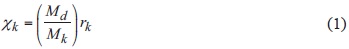
where m_k is the mass of gas k in the whole atmosphere and m_d is the total mass of the atmosphere (assuming it as dry air) with a value of 5.13 x 10²¹ g (given by Trenberth and Smith [2005] based on the atmosphere weight computed as the total surface area of the Earth multiplied by the surface pressure). Explicitly, m_k stands for the total emissions of the gas from all countries during a certain period (in this case 1990-2011), added to its mass at the beginning of the period (1990). The contributions of each country are given in its respective national inventory. M_d = 28.97 g/mol and M_k are the molecular weights of the dry air and of the k-th component, respectively. x_k in Eq. (1) is given in parts per million by volume (ppmv) for CO2 and in parts per billion by volume (ppbv) for CH₄ and N₂O. Given that the molecular weights of CO₂, CH₄ and N₂O are 44.01, 16.04 and 44.01 g/mol, respectively, we can establish from Eq. (1) the following correspondences:

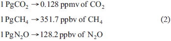
The use of equivalencies in Eq. (2) for AGG assumes that these gases, cumulated during a certain period and retained in the atmosphere are well mixed. However, the three main AGG may have an annual cycle and a horizontal gradient because they are emitted mainly in cities and industrial areas, but given that the period considered for the retained fraction of these gases in the atmosphere is 22 years (1990-2011), we can reasonably assume that they have been well mixed in the atmosphere.

 

3. The Mexican AGG emissions

An AGG inventory is usually the first step taken by a country to determine the amount and trend of AGG, in order to establish an appropriate agenda to reduce its emissions and to stop global warming. The Inventario Nacional de Gases de Efecto Invernadero (National Inventory of AGG Emissions, INEGEI) from Mexico (INECC, 2013, hereafter referred as INEGEI) covers a 21-yr period from 1990 to 2010. Given that it has specific information for each type of emission source (industry, homes, vehicles, etc.) at a municipal level, the INEGEI was prepared based on the bottom-up methodology (Ramírez, 2015) in the majority of sectors. This kind of methodology can accumulate large uncertainties in the estimation of totals for each sector, especially if the inventory is highly detailded (as TIER3 [Cruz, 2015]). The INEGEI reports a total uncertainty of ±5.6%.

The emissions of the three main AGG (CO₂, CH₄ and N₂O) shown in the INEGEI series have been practically stabilized in the last two years. Therefore, in order to quantify the contribution of Mexico to the global RF by these emissions in the period 1990-2011, we add one year to those series, assuming that emissions for 2011 were the same as in 2010. Thus, in this 22-yr period, the accumulative Mexican AGG gross emissions (before its own sinks), result in 10 276 570 Gg of CO₂, 131 830 Gg of CH₄ and 4296 Gg of N₂O.

According to the INEGEI, during 2010 ~82.1% of the CO₂ emissions came from burning fossil fuel, mainly by the energy industry. With respect to CH₄, ~49.8% was originated by fugitive emissions, largely due to the extraction of oil, coal and natural gas (this value is an uncertainty in itself, due to the emissions nature); and ~22.8% was attributable to livestock enteric fermentation. Other authors found somewhat higher percentages of this last origin: 33.7% (González and Ruiz-Suárez, 1995) and 25.4% (Castelán-Ortega et al., 2014). In the case of N₂O, 76.6% of the emissions correspond to agricultural activity, mainly soil management.

Concerning the global balance, we assume that for Mexico (as for the rest of the world), due to global sinks (which are the sum of each country's own sinks plus sinks not pertaining to any country) of these main AGG, in a sufficiently long period as 22 years, only 45.0, 3.70 and 23.2% of the emissions of CO₂, CH₄ and N₂O, respectively, are retained (and distributed homogeneously) in the atmosphere. The complement of these retentions is their sinks, the ocean being the main one. Nevertheless, before 1750 the ocean was rather a source of carbon; namely, an emission of 60.7 minus an absorption of 60.0 yields 0.7 PgC/yr During the period 2000-2009 the ocean absorbed 20 and emitted 17.7 PgC/yr, resulting in a net sink of 2.3 ± 0.7 PgC/yr. Combining the pre-industrial and industrial (present) eras, we realize that the ocean is a net sink of carbon, providing that (in PgC/yr) (60.7 + 17.7) - (60 + 20) = -1.6 (IPCC, 2013, Figure 6.1). Therefore, during the period 1990-2011 Mexico contributed to the global retention of the main AGG with 4 624 457 Gg of CO₂, 4 878 Gg of CH₄, and 997 Gg of N₂O. Taking into account the equivalences given in Eq. (2), we can estimate the corresponding concentration increases due to the emissions of a 22-yr period: 0.59 ppmv, 1.72 ppbv, and 0.13 ppbv.

 

4. Contribution of Mexico to the global radiative forcing

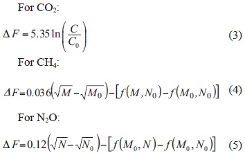
According to Myhre et al. (2013), by 2011 the global atmospheric concentrations of CO₂, CH₄ and N₂O reached 391 ± 0.2 ppmv, 1803 ± 2 ppbv, and 324 ± 1 ppbv, respectively; and the corresponding RF due to these AGG increases relative to pre-industrial values were of 1.82 ± 0.19, 0.48 ± 0.05, and 0.17 ± 0.03 Wm^-2, respectively. The IPCC (1990) gives simplified formulas to compute the RFs from Wigley (1987) with coefficients of Hansen et al. (1988) improved by Myhre et al. (1998). These formulas and coefficients are:

 

where:

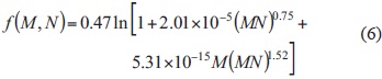
Being ΔF the RF in Wm^—2, C, M, and N are the atmospheric concentrations for 2011 of CO₂, CH₄, and N₂O, respectively; and C₀ = 278 ppmv, M₀ = 772 ppbv, and N₀=270 ppbv are the corresponding pre-industrial values. Myhre et al. (1998) determined that the uncertainties of the coefficients in Eqs. (3), (4) and (5) are 1, 10 and 5%, respectively. The logarithmic form in Eq. (3) suggests that the lines in the main CO₂ absorption band of 15 pm are mainly saturated. The cross dependence between CH₄ and N₂O in Eqs. (4) and (5) may be due to the fact that the absorption bands of these gases are partially overlapped at ~8.5 pm. The semiempirical formulas in Eqs. (3) to (5) are well established simple functional expressions, whose results for well mixed AGG are cited in the IPCC (2001, 2013). Due to their excellent agreement with explicit radiative transfer calculations, we used these formulas to compute the contribution per country to the global RF.

Hansen (1998) and the IPCC (2007, 2013) define RF as the instantaneous radiative imbalance at the tropopause. The response of the troposphere is a change in the lapse rate, keeping the tropopause temperature fixed. Eqs. (3) to (5) implicitly include water vapor with its concentration prior to the RF; in this process there are no feedbacks, and in particular vapor remains fixed.

We only estimate Mexico's contribution to the global RF for the period 1990-2011 because prior to 1990 there are no emissions inventories; so the values for this last year, denoted as ΔF*, C*, etc., are necessary. Therefore, from Eq. (3) the RF for CO₂ is:

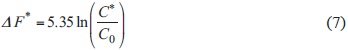
Equivalent expressions to Eq. (7) for CH₄ and N₂O can be obtained from Eqs. (4) and (5) using M* and N* instead of M and N. From Figures 2.3, 2.4 and 2.5 of the IPCC (2007), we take (for 1990): C* = 352 ppmv, M* = 1710 ppbv, and N* = 308 ppbv.

If Mexico's emissions in 1990-2011 are excluded from the rest of the world, denoted by ΔF^-, C^-, etc., we have:

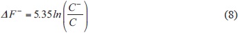
Using Mexico's contribution to the concentration increases of the three AGG (due to domestic emissions) mentioned at the end of Section 3, we obtain (for 2011): C^- = 391- 0.59 = 390.42 ppmv; whilst for CH₄ and N₂O we obtain: M^- = 1803 - 1.72 = 1801.28 ppbv and N^- = 324 - 0.13 = 323.87 ppbv, respectively.

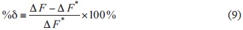
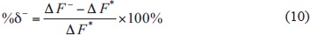
The percentage difference of RF between 1990 and 2011 is:

And without Mexican emissions:

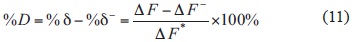
Therefore, the contribution of Mexico in absolute terms (percentage points) is given by:

And in relative terms by:

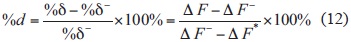
According to Eq. (9), the RF of CO₂, CH₄ and N₂O, between 1990 and 2011 increased 44.5, 7.61 and 40.2%, respectively; excluding Mexico's emissions and according to Eq. (10), these increases are of 43.9, 7.47 and 39.9%, respectively. From Eq. (11), the absolute contributions of Mexico are (%D) of 0.64, 0.14 and 0.32 percentage points, respectively, and according to Eq. (12), in relative terms (%d) they are of 1.47, 1.85 and 0.79%, respectively.

 

5. The RF of Mexico in comparison to that of Argentina, Spain and the USA

Figure II.15 of the INEGEI shows AGG emissions (specifically CO₂) and the gross domestic product (GDP), both for 2009 and per capita, for a set of 36 countries. A certain direct correlation is observed in this figure, called by us main sequence. According to this, countries with greater GDP (with the exception of the United Arab Emirates) produce greater AGG emissions; the retained fractions ofthese gases increased their concentrations in the atmosphere, and consequently the resulting RF. Within the main sequence, Mexico and the world average are at the bottom of the set with similar values, while the USA is at the top. Considering only the GDP, Spain is midway between Mexico and the USA, and Argentina is between Mexico and Spain. Thus we selected these three countries to compare their emissions and contributions to the global RF with those of Mexico.

In response to the United Nations Framework Convention on Climate Change (UN, 1992), these countries, including Mexico, elaborated their national inventories of emissions of AGG based on the year 1990, as proposed by the IPCC (1990). Spain reports its annual emissions from 1990 to 2012 (Santamarta and Higueras, 2013), with a total uncertainty of ±12.3% (DGCEAMN, 2014). Argentina reports its emissions for periods of four years, covering only the first half of the period 1990-2011: 1990, 1994, 1997 and 2000 (Fundación Bariloche, 2007), with uncertainties between ±4.0 and ±8.3% in 2000 for the sectors with highest emissions. The four annual values reported by Argentina for each gas are adjusted quite well to a logarithmic trend curve and a linear trend; we used the logarithmic (with correlations of 1.0, 0.96 and 0.92 for CO₂, CH₄ and N₂O, respectively) to determine the annual emission values of the whole period. This curve provides a more moderate increase in emissions over the 22-yr period (1990-2011) than the linear trend and a better correlation. The USA provides a table with emission values for six years: 1990, 2005, 2008, 2009, 2010 and 2011, and a histogram with annual emission values from 1990 to 2012. From these table and graph we obtained cumulative emissions for each of the three gases over the 22-yr. period. The USA inventory is highly detailed, based on the EPA methodology, and some sectors have the TIER2 level. For 2012, uncertainty in CO₂ emissions from fossil fuel combustion reaches a maximum of ±5.0%, while the uncertainty in CH₄ emissions from enteric fermentation is somewhat larger, reaching a maximum of ±18% (USEPA, 2014).

By using the warming potential per molecule ofeach AGG, we compute that 1 Gg of CH₄ is equivalent to 21 Gg of CO₂, whereas 1 Gg of N₂O is equivalent to 310 Gg of CO₂. With these data, we also compute for 2010 the per capita emissions in kilograms of equivalent CO₂ for the four countries (Table I, third column). Table I also shows, for the period 1990-2011, the percentage of each country's population compared to the world (second column); emissions retained in the atmosphere for the three AGG (fourth column), and the contribution (absolute and relative) of each country to the global RF (fifth and sixth columns, respectively).

National emissions of CH₄ and N₂O retained in the atmosphere from Argentina and Mexico are very similar, as well as their contributions to the global RF. However, CO₂ retained emissions from Argentina and their contribution to the global RF are considerably lower than those from Mexico and Spain.

Overall, the three AGG emissions per capita of Argentina, Spain and the USA represent 108.8, 110.8 and 327.0% of the Mexican ones, respectively, in units of equivalent CO₂. The CO₂ emissions of the USA retained in the atmosphere are 12.1, 19.4 and 45.0 times higher than those of Mexico, Spain and Argentina, respectively; and its relative contribution to the global RF by this gas (Table I, last column) is 14.6, 23.6 and 55.0 times higher, respectively.

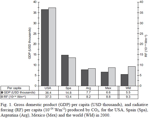
Figure 1 shows the GDP per capita in USD thousands obtained from the World Bank (http://www.worldbank.org/), as well as the RF from CO₂ in 10^-14 Wm^-2 per capita for 2000 (note that the main sequence is for 2009), which represents the middle of the period 1990-2011 in which the atmospheric retained emissions of the AGG are measured for the whole world and the four countries (USA, Mexico, Spain and Argentina). The GDP per capita in Mexico is 6.6 (in USD thousands), lower than the other countries, but somewhat greater than the world average, which is 5.5. The RF per capita of Mexico is 8.8, positioned between the RF of Argentina and Spain and practically equal to the world average, which is 9.3. Admittedly, these and former figures should have uncertainties, due to those found in the emissions inventories. The GDP data are only used as a socioeconomic context, given that our main interest is to compute Mexico's contribution to the global RF by AGG, and to compare its per capita share to those of other significant countries and with the world average.

 

6. Conclusions

Mexico contributed to the increase of the global emissions retained in the atmosphere during the 22-yr period from 1990 to 2011 with 0.59 ppmv (0.27 ppmv/decade), 1.72 ppbv (0.78 ppbv/decade) and 0.13 ppbv (0.06 ppbv/decade) of CO₂, CH₄ and N₂O, respectively.

National emissions of CH₄ and N₂O retained in the atmosphere from Argentina and Mexico are very similar, as well as their contributions to the global RF. However, CO₂ emissions from Argentina are much less than those from Mexico and Spain.

The AGG emissions per capita of Argentina, Spain and the USA are 108.8, 110.8 and 327.0% of those of Mexico, respectively, in units of equivalent CO₂. The CO₂ emissions of the USA retained in the atmosphere are 12.1, 19.4 and 45.0 times higher than those of Mexico, Spain and Argentina, respectively; and its relative contribution to the RF by this gas is, in the same order, 14.6, 23.6 and 55.0 times higher.

Mexico has a GDP per capita of 6600 USD, less than the other countries, but somewhat greater than the world average (5500 USD); its RF per capita is 8.8 x 10^-14 Wm^-2, almost equal to the world average (9.3 x 10^-14 Wm^-2) and positioned between the RFs of Argentina and Spain.

The parameters of the formulas to compute the RF from AGG concentrations have explicit uncertainties, as well as the emissions fractions retained in the atmosphere (IPCC, 2013). The main uncertainties in our estimations of Mexico's contribution to the global RF come from national emissions; in the respective inventory, we can appreciate that some sectors are not taken into account. Even though Mexico holds only 1.7% of the world population, the concentrations increase of CH₄ and N₂O due to Mexico's net emissions are similar to their respective global uncertainties: 1.72 vs. 2 ppbv and 0.13 vs. 1 ppbv.

 

Acknowledgments

We are indebted to Carlos Gay (CCA, UNAM) for reviewing the first version and his valuable comments. We also acknowledge Xóchitl Cruz (CCA, UNAM) and Fabiola Ramírez (INECC, México) for clarifying us several subjects about the INEGEI.

 

References

Castelán-Ortega O. A., J. C. Ku-Vera and J. G. Estrada-Flores, 2014. Modeling methane emissions and methane inventories for cattle production systems in Mexico. Atmósfera 27, 185-191.         [ Links ]

Ciais P., C. Sabine, G. Bala, L. Bopp, V. Brovkin, J. Canadell, A. Chhabra, R. DeFries, J. Galloway, M. Heimann, C. Jones, C. Le Quéré, R. B. Myneni, S. Piao and P. Thornton, 2013. Carbon and other biogeochem-ical cycles. In: Climate change 2013: The physical science basis. Contribution of Working Group I to the Fifth Assessment Report of the Intergovernmental Panel on Climate Change (T. F. Stocker, D. Qin, G.K. Plattner, M. Tignor, S. K. Allen, J. Boschung, A. Nauels, Y. Xia, V. Bex and P. M. Midgley, Eds.). Cambridge University Press and Environmental Protection Agency, New York.         [ Links ]

Cruz X., 2015. Personal communication. Centro de Ciencias de la Atmósfera, Universidad Nacional Autónoma de México, Mexico.         [ Links ]

DGCEAMN, 2014. Inventarios nacionales de emisiones a la atmósfera. Dirección General de Calidad y Evaluación Ambiental y Medio Natural, Ministerio de Agricultura, Alimentación y Medio Ambiente, España, 2014. Available at: http://www.magrama.gob.es/es/calidad—y—evaluacion—ambiental/temas/sistema—espanol—de—inventario—sei—/Documento_Resumen_Inventario_1990—2012_tcm7—336746.pdf.         [ Links ]

Fundación Bariloche, 2007. Segunda comunicación nacional de la República Argentina a la Convención Marco de las Naciones Unidas sobre Cambio Climático. Cap. 7. Inventario de gases de efecto invernadero de la República Argentina, no controlados por el Protocolo de Montreal. Fundación Bariloche, Argentina, pp. 52-84. Available at: unfccc.int/resource/docs/natc/ argnc2s.pdf.         [ Links ]

Garduño R. and J. Adem, 1994. Initial radiative perturbations and their responses in the Adem thermodynamic model. World Res. Rev. 6, 343-349.         [ Links ]

González E. and L. G. Ruiz-Suárez, 1995. Methane emissions from cattle in Mexico: Methodology and mitigation issues. Interciencia 20, 370-372.         [ Links ]

Hansen J., I. Fung, A. Lacis, D. Rind, S. Lebedeff, R. Ruedy and G. Russell, 1988. Global climate changes as forecast model. J. Geophys. Res. 93, 9341-9364.         [ Links ]

INECC, 2013. Inventario nacional de emisiones de gases de efecto invernadero 1990-2010. Instituto Nacional de Ecología y Cambio Climático, Secretaría de Medio Ambiente y Recursos Naturales, Mexico, 384 pp.         [ Links ]

IPCC, 1990. Climate change 1990: The scientific basis. Contribution of Working Group I to the First Assessment Report of the Intergovernmental Panel on Climate Change (J. T. Houghton, G. J. Jenkins and J. J. Ephraums, Eds.). Cambridge University Press, Cambridge, New York, Melbourne, 410 pp.         [ Links ]

IPCC, 2001. Climate change 2001: The scientific basis. Contribution of Working Group I to the Third Assessment Report of the Intergovernmental Panel on Climate Change (J. T. Houghton, Y. Ding, D. J. Griggs, M. Noguer, P. J. van der Linden, X. Dai, K. Maskell, and C. A. Johnson, Eds.). Cambridge University Press, Cambridge and New York, 881 pp.         [ Links ]

IPCC, 2007. Climate Change 2007: The Physical Science Basis. Contribution of Working Group I to the Fourth Assessment Report of the Intergovernmental Panel of Climate Change (S. Solomon, D. Qin, M. Manning, Z. Chen, M. Marquis, K. B. Averyt, M. Tignor and H. L. Miller, Eds.). Cambridge University Press, Cambridge and New York, 996 pp.         [ Links ]

IPCC, 2013. Climate change 2013: The physical science basis. Contribution of Working Group I to the Fifth Assessment Report of the Intergovernmental Panel on Climate Change (T. F. Stocker, D. Qin, G.-K. Plattner, M. Tignor, S. K. Allen, J. Boschung, A. Nauels, Y. Xia, V Bex and P. M. Midgley, Eds.). Cambridge University Press, Cambridge and New York, 1535 pp.         [ Links ]

Lee J. F. and F. W. Sears, 1962. Thermodynamics. An introduction text for engineering students. Addison-Wesley, 622 pp.         [ Links ]

Myhre G., E. J. Highwood, K. P. Shine and F. Stordal, 1998. New estimates of radiative forcing due to well-mixed greenhouse gases. Geophys. Res. Lett. 25, 2715-2718.         [ Links ]

Myhre G., D. Shindell, F.-M. Bréon, W. Collins, J. Fuglestvedt, J. Huang, D. Koch, J.-F. Lamarque, D. Lee, B. Mendoza, T. Nakajima, A. Robock, G. Stephens, T. Takemura and H. Zhang, 2013. Anthropogenic and natural radiative forcing. In: Climate change 2013: The physical science basis. Contribution of Working Group I to the Fifth Assessment Report of the Intergovernmental Panel on Climate Change (T. F. Stocker, D. Qin, G.-K. Plattner, M. Tignor, S. K. Allen, J. Boschung, A. Nauels, Y. Xia, V Bex and P. M. Midgley, Eds.). Cambridge University Press, Cambridge and New York.         [ Links ]

Ramírez F., 2015. Personal communication. Instituto Nacional de Ecología y Cambio Climático, Mexico.         [ Links ]

Santamarta J. and M. A. Higueras, 2013. Informe de emisiones de gases de efecto invernadero en España 19902012. World Wildlife Fund, Spain, 32 pp. Available at: http://awsassets.wwf.es/downloads/informe_de_emisiones_de_gei_en_espana_1990_2012.pdf.         [ Links ]

Trenberth K. E., and L Smith, 2005. The mass of the atmosphere: a constraint on global analyses. J. Climate. 18, 864-875.         [ Links ]

UN, 1992. United Nations framework convention on climate change. United Nations, New York. Available at: http://unfccc.int/essential_background/convention/items/6036.php.         [ Links ]

USEPA, 2014. Inventory of U. S. greenhouse gas emissions and sinks: 1990-2012. United States Environmental Protection Agency, Washington, DC, 528 pp. Available at: http://www.epa.gov/climatechange/emissions/usinventoryreport.html.         [ Links ]

Wigley T. M. L., 1987. Relative contributions of different trace gases to the greenhouse effect. Climate Monitor 16, 14-29.         [ Links ]