Observed surface ozone trend in the year 2012 over Nairobi, Kenya

 

ZABLON W. SHILENJE

Kenya Meteorological Department, P.O. Box 30259-00100, GPO, Nairobi, Kenya Corresponding author; e-mail: zablonweku@yahoo.com

 

VICTOR ONGOMA

Department of Meteorology, South Eastern Kenya University, P.O. Box 170-90200, Kitui, Kenya

 

Received April 27, 2014; accepted August 28, 2014

 

RESUMEN

El aire limpio es un requerimiento básico para la salud y el bienestar humanos. El Servicio Meteorológico de Kenia ha iniciado acciones de medición de contaminación del aire en varios sitios de Nairobi, en el Centro Meteorológico de Dagoretti Corner y en el monte Kenia. Se miden diversos contaminantes, incluyendo el ozono. La concentración ascendente de gases de efecto invernadero en la atmósfera ha influido en el clima y el tiempo atmosférico. En el presente estudio se analizaron las variaciones de ozono superficial en Dagoretti Corner, Nairobi, durante un periodo de 12 meses que finalizó en julio de 2013, exactamente un año después del inicio de la obtención de datos. Para estudiar la tendencia se analizaron series de tiempo horarias y mensuales de la concentración de ozono. Los datos de ozono se correlacionaron con datos meteorológicos y de temperatura. En términos generales, se encontró que la calidad del aire en Nairobi (representada por la estación meteorológica de Dagoretti Corner) es buena de acuerdo con los estándares de la Organización Meteorológica Mundial. La mayor concentración de ozono se observó durante la tarde y la mínima al amanecer. En una escala estacional, los niveles más altos se observaron en los meses fríos. Esta información ayuda a reducir la exposición al gas y por lo tanto a disminuir sus efectos sobre los seres vivos. Se recomienda la reducción de la exposición al ozono en los tiempos en que se han observado mayores concentraciones para minimizar su impacto.

 

ABSTRACT

Clean air is a basic requirement for human health and wellbeing. The Kenya Meteorological Department has established air pollution monitoring activities in various sites in Nairobi, at Dagoretti Corner meteorological station and at Mount Kenya. Different pollutants are measured including ozone. The increased concentration of greenhouse gases in the atmosphere has influenced the weather and climate. This study examined the variations of surface ozone over Dagoretti Corner, Nairobi for a 12-month period ending July 2013, exactly one year after the start of data acquisition. The trend was studied using time series analysis of ozone concentration on both an hourly and monthly basis. The ozone data was then combined with meteorological data and temperature to find correlations between the two. Overall, the air quality of Nairobi, represented by Dagoretti Corner meteorological station is good as compared to the World Meteorological Organization ozone standards. The highest concentration of ozone is observed in the afternoon and the minimum at dawn on a daily basis. On seasonal scale, the highest levels are recorded in the cold months. This information helps to reduce exposure to the gas and thus to reduce its impacts on living things. The study recommends the reduction of exposure to the gas during the times when it has been observed to be highest in order to minimize its impacts.

Keywords: Air pollution, greenhouse gas, ozone, climate, temperature, Nairobi.

 

1. Introduction

Ozone (O₃) is one of the most important global air pollutants in terms of impacts to human health, croplands and natural plant communities, and may become more important in the future. It is found in two primary layers in the atmosphere: in the upper stratosphere and the troposphere. In the upper stratosphere, it is a beneficial molecule that absorbs harmful ultra violet (UV) radiation from the sun before it reaches the Earth's surface (Crutzen, 1998). In the troposphere, ozone is a hazardous air pollutant which may cause damage to humans, animals, vegetation and materials under conditions of increasing surface ozone concentration because of smog photochemical reactions in the presence of growing atmospheric pollution (Kalabokas et al., 2000). Ozone is not directly emitted into the atmosphere; it forms as a secondary pollutant from nitrogen oxides (NO_x) and volatile organic compounds (VOCs) in the presence of sunlight. In urban areas on hot, sunny days ozone can reach very high concentration levels that can be unhealthy.

Following rapid technological and scientific advances in dynamic atmospheric chemistry processes in the recent past, air pollution monitoring has emerged as an area of research interest in different scientific institutions. This is evident in studies that have analyzed atmospheric chemicals, biogeochemical reactions (Carmichael et al., 2003) and general global circulation effects on global air pollution (Henne et al., 2008).

The increase in concentration of greenhouse gasses (GHG) in the atmosphere is central to weather and climate sensitivity and ultimately to climate change. Clean air and environment are basic requirements for human health and environmental wellbeing (WHO, 2006; NEMA, 2008). Air pollution poses an increasing threat to health and environment. According to an assessment by the World Health Organization (WHO) in 2012, over 4.3 million deaths annually are directly attributable to urban air pollution, with close 600 000 deaths in Africa (WHO, 2014).

Kenya Meteorological Department (KMD) monitors the concentration of greenhouse gases (GHG) at various sites in Kenya as one of its functions. The monitored GHGs include O₃, carbon dioxide (CO₂), carbon monoxide (CO), aerosols and particulate matter of different sizes. For almost six years, KMD only monitored vertical profiles and total column ozone using ozonesonde soundings and a Dobson spectrophotometer instrument. Since July 2012, KMD installed surface ozone analyzers specifically to measure ozone values at 10 m above the ground.

In general, ozone has not been much recorded or studied in tropical regions of the world, but it needs to be better understood since an increasing number of people around the world will be living in urban environments within the tropics. This paper examines hourly and monthly variations of surface ozone over the Dagoretti Corner meteorological station in Nairobi, for a 12-month period ending in July 2013.

Nairobi, Kenya's capital city, is located between 1° 9', 1° 28' S and 36° 4', 37° 10' E. It covers an area of 684 km² and has a population of 3.1 million people (KNBS, 2010). The predominant winds over the city are easterlies; they are associated with precipitation occasioned by moisture inflow into the country from the Indian Ocean (Opijah et al., 2007; Ongoma et al., 2013a). Nairobi has a bimodal rainfall regime with long and short rainy seasons in March-May (MAM) and October-December (OND), respectively (Okoo-la, 1996). Northeast monsoons are common during December to February, and southeast monsoons during June to August are associated to an extent with depressed rainfall conditions. Dagoretti Corner meteorological station is located at an elevation of 1795 masl, 10 km west of the central business district. Figure 1 shows the land use and location of the ozone measuring station with respect to Nairobi County.

The concentration of NOx is the main factor that determines whether O₃ forms or dissociates in the atmosphere. Ozone concentration in the troposphere is highly variable, ranging from 10 ppb (parts per billion) over the tropical oceans to 100 ppb over land, and can even exceed this last value in polluted urban areas (Denman et al., 2007). Its variability is dependent on available solar radiation, temperature fluctuations, winds, seasons and altitude, among other factors (IPCC, 2007). Atmospheric models that describe its chemistry and its coupling to transport are the best techniques currently applied to estimate current and future ozone levels.

Generally, temperature and long-term urban warming have a serious impact on urban pollution, resulting in higher ozone concentrations, since heat accelerates the chemical reactions in the atmosphere (Walcek and Yuan, 1999). Higher ozone concentration values in urban environments are mainly caused by solar radiation and pollutants. Urban areas accumulate greater amounts of heat than the surrounding rural environments, resulting in higher air temperature values in densely populated and built areas, a phenomena referred to as heat island effect (Oke, 1987). Ongoma et al. (2013b) reported that both maximum and minimum temperatures were increasing over Nairobi with the minimum increasing at a higher rate than the maximum. The increase in temperature in the cities is attributed to human activities leading to the appearance of urban heat islands (UHIs).

Bloomer et al., (2010) analyzed ozone in the eastern United States and found that its decrease was attributed to emissions reductions of its precursors and not weather variation. However, ozone has the capacity of producing feedback shocks in the climate system. According to the IPCC (2007) ozone is the third most important contributor to greenhouse radiative forcing after carbon dioxide and methane. The assessment report indicates that there was a general upward trend of carbon dioxide, methane and nitrogen oxide. According to the WMO Greenhouse Gas Bulletin (WMO, 2012), during the period 1990 through 2012, radiative forcing increased by 32% due to GHGs.

Ozone is introduced into the troposphere through its lowering down from the stratosphere. This source is most effective over oceans or regions distant from urban intensive air pollution activities (Jacob, 2000). Biomass burning also contributes to about 9% of the presence of ozone in the troposphere on a global scale. Helas et al. (1995) reported that Africa alone contributes to a substantial 40% of total global biomass burning activities. Considering the near-surface ozone concentrations, these are mainly controlled by local and regional emissions (Grewe, 2007), though they could also be affected by large-scale transport.

Ayoma et al. (2004) reported total ozone measurements over Nairobi with a Dobson instrument, confirming a maximum total ozone content during the short rainy season and a minimum in the warm-dry season. Muthama (1989) showed that minimum total ozone amount occurred around January and February (the warm-dry season) and maximum during September and October (the short rainy season).

Constant chemical reactions, such as oxidation drive the formation and destruction of ozone in the troposphere. The estimation and tracking of changes in the amounts of O₃ need measurements and actual data records. These records may be used to validate dispersion models and as a comparison to satellite data retrievals (Cui et al., 2011; Parrish et al., 2012). The Global Atmospheric Watch Program (GAW) provides reliable scientific data on the chemical composition of the atmosphere and maintains a network of stations that monitor the concentration of GHGs including ozone. Carmichael et al. (2003) describe some of the analyzers and samplers used in GAW stations.

2. Data and methodology

This study used hourly surface ozone data for a one-year period (July 2012 to July 2013) obtained from a Thermo scientific ozone analyzer model 49i. The analyzer utilizes ultraviolet radiation photometric technology to measure the amount of ozone in the sampled air in parts per billion. It is a dual photometer with both sampled and reference air flowing at the same time. Surface ozone data measurement, monitored continuously, is captured after every 2 s.

At Dagoretti Corner meteorological station in Nairobi, the analyzer is located in a laboratory room with a rainproof air inlet directed outside at a distance of 10 m above the ground. An air-sucking pump draws air into the analyzer through a filter paper that removes all particles. The filter paper is replaced every Wednesday to keep the analyzer clean.

The hourly and monthly temporal variability of ozone, as well as monthly temperature were estimated using time series analysis. The 2 s data was aggregated into hours, days, and months before calculating the annual average of 20 ppb with an 8 h highest maximum mean concentration of 30.76 ppm. The annual 8 h mean value is way below compared to the 50 ppm threshold considered by WHO to be a harmful concentration (WHO, 2006).

The predominant wind flow over Nairobi was supported by backward trajectories over this city during July 2012 and 2013. The trajectories were generated using the Hybrid Single Particle Lagrangian Integrated Trajectory Model (HYSPLIT4) complete system, in order to compute simple air parcel trajectories to complex dispersion and deposition simulations using either puff or particle approaches. The model uses previously gridded meteorological data on one of three conformal map projections (Draxler and Hess, 2010). Data are analyzed by the Global Data Assimilation System (GDAS) and are available every 12 hours. They are archived on a 2.5 * 2.5° latitude/longitude grid.

3. Results and discussion

Minimum ozone concentrations are recorded between 03:00 and 16:00 UTC (Fig. 2).

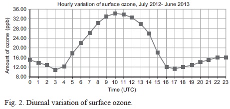
The levels of ozone concentration are observed to increase with time from 11 ppm at 03:00 UTC to 34 ppm at 10:00 UTC. A decrease in concentration is observed thereafter to 11 ppm at 17:00 UTC. The observations imply that most of the ozone at Dagoretti Corner meteorological station is thermally generated. The observed ozone concentration can thus be attributed to the prevailing weather conditions on daily to seasonal timescales.

Figure 3 shows the monthly oscillation of ozone during the study period. Maximum values of 22.5 ppm were recorded in July 2012 while the lowest concentration of 16.5 ppm was recorded in December 2012. Data within the one-year study period do not clearly reflect the seasonality.

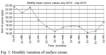
On the other hand, the lowest values were observed in December 2012, April 2013 and May 2013. These periods coincide with the rainy seasons over the study region; the long rains in March-May (MAM) and the short rains in October-December (OND). However, it is noted that ozone levels are at the lowest with a one-month lag from the onset of long rains. The results agree with studies by Ayoma et al. (2004) and Muthama (1989). The observation could therefore be attributed to wet deposition of ozone molecules, in agreement with Muralidharan et al. (1989) and Lin et al. (2009). Muralidharan et al. (1989) studied the effects of rainfall on ozone in Trivandrum, India. The study isolated a correlation between daytime rainfall and lower surface ozone levels.

During the month of July, Nairobi and its environments are under the intrusion of a cold winter air mass from the southern hemisphere that creates cloudy conditions (Opijah et al., 2007). This may also be attributed to the prevailing meteorological condition, wind. The observed concentration of ozone may have been produced in other localities and transported by wind. The attribution is in agreement with Edmonds and Basabe (1989). Figure 4 shows a 168-h backward air trajectory ending at 00:00 UTC, on July 15, 2012 and July 15, 2013.

The predominant flow at the mentioned times over Nairobi is southeasterly, which is in agreement with Opijah et al. (2007) and Ongoma et al. (2013a).

The monthly ozone concentration has a negative correlation with temperature over the same period (Fig. 5). The correlation coefficient between the two variables is -0.13.

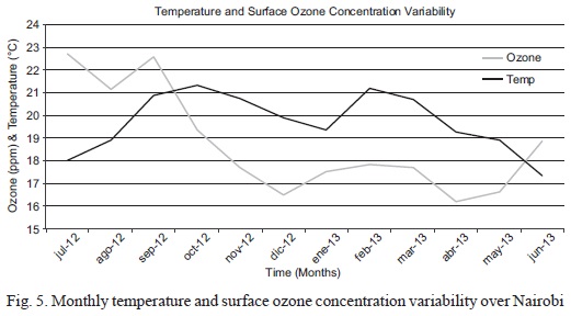
The negative correlation coefficient indicates that the variation of monthly ozone concentration is inversely proportional to temperature in the area of study. The cold and dry season of June-August (JJA) is thus expected to have a high ozone concentration; conversely, the hot and dry months of December-February (DJF) are expected to have the lowest concentration of ozone. The observation differs from some studies (e.g. Solberg et al., 2005) in other localities where pho-tolytic reactions leading to ozone formation increase with temperature and O3 production is generally at its maximum during warmer sunny weather. According to Solberg et al. (2005), the measurements of a study carried out in Southern England during 1995 showed an annual cycle of ozone with an early summer peak of about 40 ppb and an autumn minimum of about 25 ppb. When superimposed on the annual cycle substantial variations were evident from day to day, with peaks of up to 200 ppb on sunny warm days and minima on cold calm winter days, when dry deposition to the surface exceeds the supply of O₃ from aloft.

Since wind direction and speed are very important in determining the concentrations of O3 precursors within a region, the high concentration of ozone during JJA can be attributed to the strong southeasterly monsoon that flows over the city.

4. Conclusion and recommendations

Although the surface ozone monitoring station at Dagoretti Corner in Nairobi is still in its early stages, it shows the trends of the collected data. On a daily basis, the highest concentration of ozone is observed during the afternoon and the minimum at dawn. On a seasonal scale the highest levels are recorded during cold months, which is attributed to the rain-wash of pollutants during the wet months. Air pollution that contributed to the highest levels of ozone on specific days may not have come from a particular area, implying that pollution may come from many directions, a fact that policy makers should take into account. It is worth noting that the highest surface ozone concentration at the Dagoretti Corner meteorological station is almost twice lower than the WHO highest recommended threshold of 50 ppm.

Surface ozone data collection and analysis will provide important information to stakeholders with reference to the key components of its location, concentration and expected impacts. This information helps reducing exposure to the gas and thus diminishes its impacts on living things. The study recommends reducing exposure to the gas during times when it has been observed to be highest, in order to minimize its impacts. The study also recommends the continuous and accurate observation of surface ozone in the area of study for further research in the area.

Acknowledgements

We are grateful to our colleagues Messers, K. Thiong'o, J. M. Kariuki and J. K. Nguyo for the facilitation of data collection. We are also appreciative to our respective institutions and MeteoSwiss, which supported the installation and operation of the surface ozone analyzer at Dogoretti, Nairobi.

 

References

Ayoma W., L. Gilbert and C. Bertrand, 2004. Variability in the observed vertical distribution of ozone over equatorial Eastern Africa: An analysis of Nairobi ozonesonde data 2004. Proceedings of the Quadrennial Ozone Symposium, 1-8 June, Kos, Greece.         [ Links ]

Bloomer B. J., K. Y. Vinnikov and R. R. Dickerson, 2010. Changes in seasonal and diurnal cycles of ozone and temperature in the Eastern U.S. Atmos. Environ. 44, 2543-3551.         [ Links ]

Carmichael G. R., M. Ferm, N. Thongboonchoo, J. H. Woo, L. Chan, K. Murano and J. Boonjawat, 2003. Measurements of sulfur dioxide, ozone and ammonia concentrations in Asia, Africa, and South America using passive samplers. Atmos. Environ. 37, 1293-1308.         [ Links ]

Crutzen P. J., 1998. How the atmosphere keeps itself clean and how this is affected by human activities? Pure Appl. Chem. 70, 1319-1326.         [ Links ]

Cui J., D. S. Pandey, M. Sprenger, S. Henne, J. Staehelin, M. Steinbacher and P. Nedelec, 2011. Free tropospheric ozone changes over Europe as observed at Jungfraujoch (1990-2008): An analysis based on backward trajectories. J. Geophys. Res.-Atmos. 116, 1984-2012.         [ Links ]

Denman K. L., G. Brasseur, A. Chidthaisong, P. Ciais, P. M. Cox, R. E. Dickinson, D. Hauglustaine, C. Heinze, E. Holland, D. Jacob, U. Lohmann, S. Ramachandran, P. L. da Silva Dias, S. C. Wofsy and X. Zhang, 2007. Couplings between changes in the climate system and biogeochemistry. In: Climate change 2007: The physical science basis. Contribution of Working Group I to the Fourth Assessment Report of the Intergovernmental Panel on Climate Change (S. Solomon, D. Qin, M. Manning, Z. Chen, M. Marquis, K. B. Averyt, M. Tignor and H. L. Miller, Eds.). Cambridge University Press, pp. 499-588.         [ Links ]

Draxler R. R. and G. D. Hess, 2010. Hybrid single-particle Lagrangian integrated trajectories (HY-SPLIT): Version 4.0 - Description of the Hysplit_4 Modeling System. NOAA Technical Memorandum ERL ARL-224, 27 pp.         [ Links ]

Edmonds R. L. and F. A. Basabe, 1989. Ozone concentrations above a douglas-fir forest canopy in Western Washington, U.S.A. Atmos. Environ. 23, 625-629.         [ Links ]

Grewe V., 2007. Impact of climate variability on tropospheric ozone. Sci. Total Environ 374, 167-181.         [ Links ]

Helas G., J. Lobert, D. Scharffe, L. Schäfer, J. Goldammer, J. Baudet and R. Delmas, 1995. Airborne measurements of savanna fire emissions and the regional distribution of pyrogenic pollutants over Western Africa. J. Atmos. Chem. 22, 217-239.         [ Links ]

Henne S., J. Klausen, W. Junkermann, J. Kariuki, J. Aseyo and B. Buchmann, 2008. Representativeness and climatology of carbon monoxide and ozone at the global GAW station Mt. Kenya in equatorial Africa. Atmos. Chem. Phys. 8, 3119-3139.         [ Links ]

IPCC, 2007. Synthesis report. Contribution of working group I, II and III to the Fourth Assessment Report of the Intergovernmental Panel on Climate Change (R. K. Pachauri and A. Resinger, Eds.). IPCC, Geneva, Switzerland, 104 pp.         [ Links ]

Jacob D. J., 2000. Heterogeneous chemistry and tropospheric ozone. Atmos. Environ. 34, 2131-2159.         [ Links ]

KNBS, 2010. The 2009 Kenya population and housing census. Kenya Ministry of State for Planning, National Development and Vision 2030. Government Print Press, Nairobi, 297 pp. Available at: http://www.knbs.or.ke/index.php?option=com_phocadownload&view=category&id=109:population-and-housing-census-2009&Itemid=599.         [ Links ]

Lin M., T. Holloway, T. Oki, D. G. Streets and A. Richter, 2009. Multi-scale model analysis of boundary layer ozone over East Asia. Atmos. Chem. Phys. 9, 3277-3301.         [ Links ]

Makokha G. L. and C. A. Shisanya, 2010. Trends in mean annual minimum and maximum near surface temperature in Nairobi City, Kenya. Advances in Meteorology, doi:10.1155/2010/676041.         [ Links ]

Muralidharan V., G. M. Kumar and S. Sampath, 1989. Surface ozone variation associated with rainfall. Pure Appl. Geophys. 130, 47-55.         [ Links ]

Muthama N. J., 1989. Total atmospheric ozone characteristics over a tropical region. MSc thesis. Department of Meteorology, University of Nairobi, Kenya.         [ Links ]

Kalabokas P. D, L. G. Viras, J. Bartzis and C. C. Repapis, 2000. Mediterranean rural ozone characteristics around the urban area of Athens. Atmos. Environ. 34, 5199-5208.         [ Links ]

NEMA, 2008. The environmental management and coordination (air quality) regulations. National Environment Authority, Nairobi, Kenya.         [ Links ]

Oke T. R., 1987. Boundary layer climates, 2^nd ed. Routledge, London and New York, 464 pp.         [ Links ]

Okoola R. E., 1996. Space-time characteristics of the ITCZ over equatorial Eastern Africa during anomalous rainfall years. Ph.D. thesis. Department of Meteorology, University of Nairobi, Kenya.         [ Links ]

Ongoma V., J. N. Muthama and W. Gitau, 2013a. Evaluation of urbanization influences on urban winds of Kenyan cities. Ethiopian Journal of Environmental Studies and Management 6, 223-231.         [ Links ]

Ongoma V., N. J. Muthama and W. Gitau, 2013b. Evaluation of urbanization influences on urban temperature of Nairobi City, Kenya. Global Meteorology 2, doi:10.4081/gm.2013.e1.         [ Links ]

Opijah F. J., J. R. Mukabana and J. K. Ng'ang'a, 2007. Rainfall distribution over Nairobi area. J. Meteorol. Rel. Sci. 1, 3-13.         [ Links ]

Parrish D., K. S. Law, J. Staehelin, R. Derwent, O. Cooper, H. Tanimoto and M. Steinbacher, 2012. Long-term changes in lower tropospheric baseline ozone concentrations at northern mid-latitudes. Atmos. Chem. Phys. 12, 11485-11504, doi:10.5194/acp-12-11485-2012.         [ Links ]

Solberg S., R. G. Derwent, 0. Hov, J. Langner and A. Lindskog, 2005. European abatement of surface ozone in a global perspective. Ambio 34, 47-53.         [ Links ]

Walcek C. J and H. H. Yuan, 1999. Calculated influence of temperature-related factors on ozone formation rates in the lower troposphere. J. Appl. Meteorol. 34, 1056-1069.         [ Links ]

WHO, 2006. Air quality guidelines: Global update 2005. Particulate matter, ozone, nitrogen dioxide and sulphur dioxide. World Health Organization Regional Office for Europe, Copenhagen, 484 pp.         [ Links ]

WHO, 2014. Burden of disease from household air pollution for 2012. World Health Organization, Geneva. Available at: http://www.who.int/phe/health_topics/outdoorair/databases/FINAL_HAP_AAP_BoD_24March2014.pdf?ua=1 (last accessed on March 15, 2014).         [ Links ]

WMO, 2012. The state of greenhouse gases in the atmosphere, based on global observations through 2012. WMO Greenhouse Gas Bulletin 9. Available at: http://www.wmo.int/pages/prog/arep/gaw/ghg/documents/GHG_Bulletin_No.9_en.pdf.         [ Links ]