Climate downscaling over southern South America for present-day climate (1970-1989) using the MM5 model. Mean, interannual variability and internal variability

 

FERNANDA CABRÉ

Centro de Investigaciones del Mar y la Atmósfera (CIMA-CONICET/FCEN-UBA); Instituto Franco Argentino de Estudios del Clima y sus Impactos (UMI IFAECI/CNRS) Ciudad Universitaria, pabellón II, piso 2, C1428EGA, Buenos Aires, Argentina. Corresponding author; e-mail: cabre@cima.fcen.uba.ar

 

SILVINA SOLMAN and MARIO NÚÑEZ

Centro de Investigaciones del Mar y la Atmósfera (CIMA-CONICET/FCEN-UBA); Departamento de Ciencias de la Atmósfera y los Océanos (DCAO/FCEN-UBA); Instituto Franco Argentino de Estudios del Clima y sus Impactos (UMI IFAECI/CNRS), Ciudad Universitaria, pabellón II, piso 2, C1428EGA, Buenos Aires, Argentina

 

Received March 26, 2013; accepted November 26, 2013

 

RESUMEN

Este trabajo evalúa la capacidad del modelo regional MM5 para representar las principales características del clima actual de Sudamérica. Se evalúa la distribución espacial de los valores medios estacionales, la variabilidad interanual y el ciclo anual de la precipitación y la temperatura, así como la variabilidad interna. El análisis tuvo dos objetivos: cuantificar la capacidad de la regionalización (downscaling) dinámica para representar el clima actual e identificar los aspectos críticos de la simulación climática regional en Sudamérica para interpretar las proyecciones hacia fines de siglo XXI en el escenario de emisión SRES A2 con cierto grado de confiabilidad. En general, el modelo MM5 representa de forma adecuada las características regionales, el ciclo estacional y la variabilidad interanual de las variables de superficie en el sur de Sudamérica. La distribución espacial de la temperatura está bien representada; sin embargo, se encuentran algunos errores sistemáticos, como una sobreestimación en el centro y norte de Argentina y una subestimación en las regiones montañosas a lo largo del año. La distribución espacial de la precipitación también está bien representada por el modelo regional, sin embargo se encuentra una sobreestimación de la precipitación en la región andina (especialmente en el centro y sur de Chile) en todas las épocas del año y una subestimación de la precipitación en latitudes tropicales. El ciclo anual de la precipitación está representado de manera adecuada en todas las regiones analizadas, sin embargo su representación es mejor en la cuenca del Plata (LPB, por sus siglas en inglés), Cuyo (CU) y sur de Buenos Aires (región denominada sureste Pampas [SEP]). El ciclo anual de la temperatura media también está bien representado. En líneas generales, el modelo sobreestima la variabilidad interanual de la temperatura y subestima la variabilidad interanual de la precipitación. De la evaluación de la variabilidad interanual, la variabilidad interna y los sesgos, puede concluirse que independientemente de la época del año, la precipitación simulada por el modelo regional MM5 es confiable en latitudes subtropicales, Uruguay, el sur de Brasil y el centro-este de Argentina, pero es poco confiable en áreas montañosas. La temperatura es confiable en latitudes subtropicales, Uruguay y el sur de Brasil solamente durante el invierno, pero es poco confiable o se encuentra en el límite de confiabilidad en el centro y sur de Chile a lo largo del año. De esta manera, puede concluirse que el modelo MM5 es una herramienta de mucha utilidad para la generación de escenarios regionales de cambio climático de alta resolución en el sur de Sudamérica y constituye un interesante punto de partida para evaluar los escenarios regionales de cambio climático en dicha región.

 

ABSTRACT

This work focuses on evaluating the ability of the MM5 regional model to represent the basic features of present climate over South America. The spatial distribution of seasonal means and the interannual variability, as well as annual cycles for precipitation and near-surface temperature have been evaluated. The internal variability has also been investigated. The analysis has two objectives: one of them is to quantify the dynamic downscaling ability to represent the current climate and the other is to identify critical aspects of the regional climate model in South America in order to interpret the reliability of future projections for the end of the twenty-first century in the A2 scenario of the IPCC Special Report on Emissions Scenarios. In general, the MM5 model is able to reproduce adequately the main general features, seasonal cycle and year-to-year variability of near surface variables over South America. The spatial distribution of temperature is well represented, but some systematic errors were identified, such as an overestimation in central and northern Argentina and an underestimation in the mountainous regions throughout the year. The general structure of precipitation is also well captured by the regional model, although it overestimates the precipitation in the Andean region (specifically in central and southern Chile) in all seasons and underestimates the rainfall over tropical latitudes. The annual cycle of precipitation is adequately represented in the subregions analyzed, but its representation is better over La Plata basin (LPB), Cuyo (CU) and southeastern Pampas (SEP). The annual cycle of mean temperature is well represented, too. The model systematically overestimates the interannual variability of temperature and underestimates the interannual variability of precipitation. From the analyses of interannual and internal variability, as well as the biases, it can be concluded that regardless the season, the simulated precipitation is reliable at subtropical latitudes, Uruguay, southern Brazil and east-central of Argentina, but is less reliable over areas of complex topography. For temperature, the regional model is reliable over subtropical latitudes, Uruguay and the south of Brazil only during winter, but it is less reliable or it is even in the limit of reliability over central and southern Chile all along the year. Therefore, it is concluded that the MM5 model is a useful tool for the generation of regional climate change scenarios and for the evaluation of regional climate change scenarios over southern South America.

Keywords: Regional climate modeling, South America, present climate, interannual variability, internal variability, ensemble.

 

1. Introduction

General circulation models (GCMs) are the most promising tools to determine the response of the climate system to increasing greenhouse gases concentrations and to assess how the system will evolve under different emission scenarios. Nevertheless, due to the complexity of these models and the fact that they operate globally, their spatial resolution, typically of several hundred kilometers, is considered insufficient for many purposes. First of all, GCMs are not able to adequately capture the regional scale forcing and, in consequence, they are not able to represent the small-scale processes and their related heat and momentum fluxes that critically affect the broader scale circulation. Moreover, near-surface variables are strongly influenced by local and regional forcings, which cannot be properly represented due to the spatial resolution in which the model operates.

The development of regional climate models (RCMs) nested in GCMs has been extensively used for different applications and regions since the early 1990s (Dickinson et al. 1989; Giorgi, 1990). Nowadays, regional climate modeling is the most appropriate tool to simulate the regional climate with greater accuracy than the low-resolution global models, accounting for small-scale features related to thermal contrasts due to complex topography or other inhomogeneities at surface. Studies such as Caya and Biner (2004), Giorgi et al. (2004) and Raisanen et al. (2004) show that RCMs improve the representation of climate variables such as precipitation and surface temperature when compared with GCMs.

Regional climate modeling studies over South America have shown a diverse model performance, depending on the choice of the regional model (Rauscher et al. 2006; Seth et al. 2007; Alves and Marengo 2009; Chou et al. 2009, 2012; Silvestri et al. 2009; Menéndez et al. 2010a,b; Sorensson et al. 2010). Solman et al. (2007) explored the capability of the MM5 model to reproduce the main features of present climate over the region. In addition, several studies have evaluated the quality of present-climate simulations using different RCMs nested into the HadAM3P global model (Alves and Marengo (2009) using the HadRM3P; da Rocha et al. (2009) using the RegCM3; Pisnichenko and Tarasova (2009) using the Eta CCS; and Pesquero et al. (2009) using the Eta-CPTEC RCMs). When compared with observations, the regional simulations exhibit systematic errors that might be related to the physics of RCMs (e.g., convective schemes and land surface processes) and the lateral boundary conditions inherited from the global model.

The application of ensembles of RCMs simulations to assess the significance of model perturbations began in the early 1990s (Ji and Vernekar, 1997; Rin-ke and Dethloff, 2000; Weisse et al., 2000; Gaertner et al., 2001). Besides this, several studies have shown that regional climate simulations are affected by various sources of uncertainty (de Elia et al., 2008) and the spread among different simulations should be borne in mind before drawing conclusions about the significance of the regional climate model response to external forcings. O'Brien et al. (2010) provides a very clear example of this behavior.

The sources of uncertainty in regional climate simulations can be classified in four groups: (a) uncertainty due to differences in initial conditions, known as internal variability (IV); (b) uncertainty due to the model configuration (e.g., domain size and location); (c) uncertainty due to the choice of physical parameterization in the RCM; and (d) uncertainty due to the boundary conditions (driving global climate models and/or reanalysis). In addition to the above classification, in simulations where we evaluate the response to increasing concentrations of greenhouse gases, the uncertainty of the scenario represents an additional source of uncertainty (Hawkins and Sutton, 2009).

Internal variability is related to differences among realizations of the simulated climate triggered by distinct initial conditions. Consequently, the internal variability tries to account for the intrinsic uncertainty in the simulated climate (von Storch, 2005). It has been shown that RCMs have some level of freedom and therefore show an important IV (Giorgi and Bi, 2000; Christensen et al., 2001; Caya and Biner, 2004; Alexandru et al., 2007). Moreover, it has been shown that IV is sensitive to the simulated period, the domain size and geographic location. This has motivated several studies focused on evaluating IV, such as those that aim for assess the magnitude of IV in RCMs and characterize both spatial and temporal distribution, as well as its dependence on the number of ensemble members and the domain size (Giorgi and Bi, 2000; Christensen et al., 2001 over the Mediterranean region, southern Europe and northern Africa; Caya and Biner, 2004; Alexandru et al., 2007; Lucas-Picher et al., 2008 in North America; Vanvyve et al., 2008 for western Africa; and Solman and Pessacg, 2012a for South America). Moreover, the IV represents the lowest level of uncertainty that cannot be reduced, but should be characterized in order to assess the extent to which the response of the regional climate represents a significant signal or is immersed in the inherent uncertainty of the RCM.

Although the literature related to IV in other parts of the world is extensive, South America does not show that privilege. There are no studies focused on evaluating the magnitude of the uncertainties of long-term RCM simulations over the region. Solman and Pessacg (2012b) have evaluated the behavior of several uncertainty sources for South America at the seasonal scale. We propose studying and quantifying the IV in the MM5 RCM for a one-year simulation in order to discuss the limitations of the model, by comparing its biases with the IV.

Southern South American climate and its variability are affected by regional and local forcings. The target region extends from the tropics towards the extratropics and high latitudes, the southernmost part of the region being embedded within the westerly circulation. Climate over this region is characterized by interactions of several dynamical processes. The most important feature of the regional geography is the Andes Mountains, a very narrow orographic feature extending all along the western coast which reaches up to 6000 m at subtropical latitudes. In addition, the Brazilian plateau, covering most of eastern Brazil is another important topographic structure in the continent. Both mountainous systems produce distinctive features in the South American climate, particularly at low levels. The presence of a low level jet along the eastern slopes of the central Andes as well as the existence of a region of maximum frequency of winter cyclogenesis over eastern South America, are examples of the topographic influence on the continental climate (Vera et al. 2006 and references therein).

The first step to understand climate changes that are likely to occur in the future is the assessment of present climate. Such an assessment also allows determining the model deficiencies, among other topics. For this reason, this paper provides an evaluation ofa present climate simulation over southern SouthAmerica performed with the MM5 regional model. We focus on evaluating the capability ofthe model in reproducing the seasonal mean climate and the interannual variability for precipitation and near-surface temperature. This article is an initial step for further evaluating the regional climate response under the A2 scenario of the IPCC Special Report on Emissions Scenarios over the region, to be used for impact studies over South America.

This paper is organized as follows: section 2 presents some characteristics of the MM5 RCM in terms of its configuration, experiment design and validation data. A brief detail of the climate indices of IV is also presented in this section. Section 3 is devoted to assessing the performance of the regional model. We evaluate the low-level circulation patterns in terms of the spatial distribution of wind and its meridional component. Then we discuss the spatial distribution of seasonal mean temperature and precipitation, the annual cycle and the interannual variability. A brief evaluation of the MM5 IV for both temperature and precipitation is also included. Section 4 aims to discuss the reliability of the simulation. The objective of this analysis is to put the mean seasonal biases in the context of interannual and internal variability, for evaluating the extent to which the model is able to reproduce a reliable estimate of present climate conditions. Finally, section 5 summarizes the conclusions.

 

2. Model description, experiment design and validation data

2.1 The regional model

The regional climate simulation was performed using the fifth-generation Pennsylvania State Universi-ty-NCAR nonhydrostatic Mesoscale Model MM5 version 3.6, developed by Pennsylvania State University (PSU) and the National Centers for Environmental Prediction/National Centre for Atmospheric Research (NCEP/NCAR) (Grell et al., 1993).

The regional model configuration used to perform the continuous 20-year simulation for the period 1970-1989 includes the Grell convective scheme (Grell et al., 1993). The planetary boundary layer parameterization is formulated following the MRF scheme by Hong and Pan (1996). Surface processes are represented by the Noah land surface model (Chen and Dudhia, 2001). Moisture tendencies were calculated by the explicit moisture scheme (Hsie et al., 1984). The radiation package calculates long-wave radiation through clouds and water vapor, based on Stephens (1978, 1984) and Garrand (1983). It also accounts for short wave absorption and scattering in clear air, and reflection and absorption in cloud layers (Stephens, 1984). The calculation of radiative heating or cooling in the atmosphere accounts for longwave and shortwave interactions with explicit cloud and clear air. The non-hydrostatic dynamics allows the model to be used effectively in representing phenomena with very high resolution.

The regional model was run in a Mercator grid with approximately 40 km resolution in both horizontal directions, with 158 points in the west-east direction and 150 points in the south-north direction, with 23 vertical sigma levels. The land-sea mask and topography have been derived from the US Navy 10 min resolution dataset. Vegetation and soil properties were obtained from the U.S. Geological Survey (USGS) vegetation/land use database. The integration domain covers southern South America, from 12° to 58° S, 28° to 92° W. Figure 1 displays the model topography and domain used in this study.

2.2 Boundary conditions and experiment design for climate simulations

Data from the Atmospheric GCM HadAM3H developed by the Hadley Center was used to drive the MM5 regional model. The HadAM3H model resolution is 1.25° latitude by 1.875° longitude. Details ofthe model characteristics can be found in Pope et al. (2000). The HadAM3H present-climate simulations from 1961 to 1990 were initialized with atmospheric and land surface conditions from the Coupled Ocean-Atmosphere Global Climate Model (HadCM3) and forced with observed sea surface temperature (SST) and sea-ice distribution from the Hadley Centre HadISST dataset (Rayner et al., 2003). This database shows a mixture of global monthly sea surface temperature and sea-ice concentration at 1° horizontal resolution from 1871.

The MM5 model requires initial and time evolving boundary conditions for wind components, temperature, geopotential height, relative humidity and surface pressure. These variables were provided in a 6-hour interval within a relaxation zone in the lateral boundaries.

The model integration started on January 1, 1969 and the simulation extends up to December 30, 1989. A one-year spin-up time was adopted (Christensen, 1999), which was excluded for the analysis.

2.3 Methodology and experimental design for ensemble analysis

A three-member ensemble for a one year-length simulation (1987) has been performed. Each member shares the same experimental design (model configuration, lateral boundary conditions and physical schemes) with the only exception that the initial condition is different among them.

The design of the proposed experiment consists of modifying the initial condition by changing the starting day for each member of the ensemble. The analysis was conducted from December 1, 1986 to December 1, 1987. The three-member ensemble is called EXP1-EXP2-CTL. Table I specifies the name of each member together with the corresponding initial condition.

We also carried out three other ensembles of two members (EXP1-EXP2, EXP1-CTL, EXP2-CTL), in order to perform a brief sensitivity analysis to the number of members of the ensemble.

2.4 Climate statistics of internal variability A measure of the uncertainty for each ensemble is quantified by means of the spread among the ensemble members, using the variance estimated between each three-member ensemble as in Alexandru et al. (2007):

where M is the number of ensemble members (M = 3); X_m(i, j, t) represents the value of the variable X (temperature or precipitation) at grid point (i, j) at time t, for the individual ensemble member m; and (X ^(i, j, t) represents the ensemble mean, defined as:

The temporal evolution of IV can be obtained with the areal average of σ²_VAR expressed by:

where VAR represents the variable evaluated (temperature or precipitation), and I and J specify the number of points in the x and y directions, respectively.

As a measure of the spatial distribution of the spread among individual members of the ensembles (IV), we computed the square root of the time-averaged variance:

where N is the number of time-steps of the simulated period. The last equation represents the climatology of IV at an individual grid point (i, j).

These statistics will be evaluated for precipitation and surface air temperature at the seasonal scale.

2.5 Validation data

For the validation of monthly mean precipitation and surface air temperature, the Climate Research Unit (CRU) dataset (Mitchell et al., 2003) from East Anglia University has been used. CRU is available over a 0.5° x 0.5° horizontal grid. The NCEP/NCAR reanalysis (Kalnay et al., 1996) was used for validation of the circulation variables (zonal and meridional winds).

 

3. Results

The results focus on present climate features (19701989) for austral summer (DJF), fall (MAM), winter (JJA) and spring (SON).

3.1 Mean climate

3.1.1 Validation of low-level circulation patterns Figure 2 shows the seasonal circulation of the lower troposphere together with the spatial distribution of the meridional component of wind for summer (DJF) and winter (JJA), both from the HadAM3H global model (left column), the MM5 regional model (middle column), and the NCEP/NCAR reanalysis (right column) (Kalnay et al., 1996).

One of the main features of the summer circulation over South America is the low-level jet (LLJ) along the eastern slope of the Andes. The center of this LLJ is located approximately at 850 hPa and 17° S (Saulo et al., 2000). At subtropical latitudes, the Andes act as a barrier to the low-level atmospheric flow from the Pacific Ocean. Southward of 45° S the mountains are lower and the flow over the continent is dominated by westerlies from the Pacific. Comparing the upper and lower right panels of Figure 2, it can be seen that the NCEP/NCAR reanal-ysis displays a more intense LLJ for winter compared to summer months, as expected.

With respect to the spatial distribution of wind, during DJF over subtropical South America, the NCEP/NCAR reanalysis exhibits an anticyclonic circulation from the Atlantic Ocean (about 2 to 4 m/s) and a circulation from tropical latitudes along the eastern slope of the Andes (about 4 to 6 m/s). An anticyclonic gyre over the Pacific Ocean northward of 40° S, with intensities between 5 and 8 m/s is also apparent. South of 40° S the magnitude of the westerly wind is of the order of 9 to 12 m/s. In general, the MM5 regional model adequately represents the features described above. However, there are some differences between modeled and reanalysis data. During DJF, the regional model underestimates the wind at 850 hPa by around 3 m/s over the Pacific Ocean. The wind at 850 hPa on the eastern slope of the Andes shows the same intensity that the observed values (between 4 to 6 m/s), while the anticyclonic circulation from the South Atlantic Ocean is overestimated. The regional model also overestimates the wind over the Patagonian region.

The spatial distribution of the wind for winter months is very similar to that for summer, but it presents a northward displacement (5° on average) and is weaker compared with summer values. Intensities between 1 and 3 m/s are observed in the anticyclonic gyre circulation from the Atlantic Ocean, while slightly higher intensities (between 4 and 6 m/s) are seen in the anticyclonic circulation of the Pacific Ocean. South of 40° S, the intensities do not exceed 10 m/s. The simulated wind at 850 hPa presents lower values than those observed over the Pacific Ocean. The wind from tropical latitudes is underestimated (about 1 to 3 m/s). South of 40° S, intensities are 10 m/s and 11 m/s, indicating a slight overestimation with respect to the reanalysis.

The spatial distribution of the meridional component of the wind at low levels during DJF shows two major areas, one located east of 65° S and north of 35° S characterized by negative values (southward direction), and the other located over the Pacific coast with positive values (northward direction). These features are generally well reproduced by both regional and global models; however, the northward wind over the Pacific coast is closer to the continent in the models compared to the reanalysis. The regional model improves the representation of flow from the northern Amazon region east of the Andes compared with the global model, though the regional model slightly overestimates the intensity over west-central Argentina and southern Bolivia.

During winter months the regional model underestimates the meridional component of wind at 850 hPa over the region located east of 65° S and north of 35° S. The lower panels in Figure 2 show that according to the NCEP/NCAR reanalysis the intensity of meridional wind from the north exceeds -5 m/s, while the regional model simulated intensities are of the order of -2 to -3 m/s. It is important to note that the regional model presents a strong southward component over this area, while the reanalysis has a southeastward direction.

The inadequate representation of the Chaco low in the global model (not shown) may explain why the northerly wind extends too far southwards compared with the reanalysis. The regional model captures reasonably well the structure of the LLJ over Bolivia, but the cyclonic circulation associated with the Chaco low is displaced to the northeast. Due to this misrepresentation of the circulation at low levels, the wind over Paraguay, southeastern Brazil, northeastern Argentina and Uruguay shows an important bias in the regional model.

Overall the MM5 regional model adequately captures the characteristics of circulation in the lower troposphere (in terms of wind direction and intensity, as well as the magnitude and location of the maxima of meridional wind). It is important to note that using the Grell convection scheme some model deficiencies were improved with respect to the results documented in Solman et al. (2007).

3.1.2 Validation of surface variables for present climate (1970-1989)

Figure 3 compares the 20-year mean seasonal precipitation from the regional model (left column), CRU observations (middle column) and the differences between them (right column) for summer (DJF), autumn (MAM), winter (JJA) and spring (SON).

During summer (the wet season for most of South America east of the Andes) large precipitation associated with the South American Monsoon System and the South Atlantic Convergence Zone (SACZ) (Kodama, 1992), located over southeastern Brazil are apparent. Over this area observed precipitation ranges from 8 to 10 mm/day whereas lower intensities (from 4 to 8 mm/day) are observed over the south of Brazil, Paraguay, and the center and northeast of Argentina. The MM5 regional model is capable of reproducing these features and also captures low precipitation rates over the Patagonian region. However, it is important to note that the maximum precipitation associated with the SACZ is underestimated by around 3 mm/day. The systematic underestimation of precipitation in tropical areas with the Grell scheme has also been documented by Solman and Pessacg (2012a) with the MM5 regional model, by Fernández et al. (2006) and da Rocha et al. (2009) with the RegCM3 regional model, and by Chou et al. (2012) with the Eta regional model.

While the MM5 model captures the observed maximum of precipitation in areas of high topography, its magnitude is overestimated. Similar features have been reported in different studies of regional climate modeling in South America using the RegCM3, EtaClim and PRECIS regional models (Fernández et al., 2006; Marengo et al., 2009b). This shortcoming has also been documented in other mountainous regions in South America and elsewhere in the world with the MM5 regional model, including Rojas (2006) in central Chile and Grell et al. (2000) in the Alps, respectively.

During winter (dry season), CRU displays values below 1 mm/day over most parts of Argentina, northern Chile and southwestern Bolivia; except at the easternmost region of Argentina, Uruguay and southern Brazil where a maximum of precipitation is apparent. During this season the areas with largest rainfall amounts (from 4 to 6 mm/day) were found over southern Brazil and Uruguay (as a result of the frontal activity) and over central and southern Chile (ranging from 8 to 10 mm/day).

Overall, the spatial distribution of the modeled winter precipitation is very similar to observations. The MM5 model adequately represents the dry conditions over most of the region, except over Uruguay and southeastern Brazil. Though the regional model captures the maximum precipitation, its magnitude is underestimated by around -4 mm/day. This underestimation is also present in the 10-year simulation documented in Solman et al. (2007) with the same model.

In general the geographical distribution of modeled and observed rainfall is very similar. The regional model underestimates the precipitation amount over the center-east of Argentina, Uruguay and south of Brazil. The underestimation of rainfall is larger during spring than during fall; during summer the model shows the largest negative biases. It is important to note that underestimation associated with SACZ is also present during the transition seasons. The southern tip of the continent displays the opposite pattern, in which simulated precipitation is larger than the observed over the western slope of the Andes.

As mentioned above the maximum observed precipitation over the central and southern part of Chile shows a latitudinal displacement during the year, with intensities of around 6 mm/day in both fall and spring. The regional model adequately reproduces the latitudinal distribution and meridional shift of the maximum precipitation, but the magnitude is always overestimated (because of stronger westerly winds interacting with the western slope of the Andes [Solman et al., 2007]). A larger overestimation of rainfall is found during winter months, with a positive bias of about 6 mm/day. The positive bias in precipitation is a common feature of regional climate simulations in areas of high topography. Similar results with the MM5 regional model have been found in Grell et al. (2000) for the Alps and Rojas (2006) for central Chile. Large overestimate of rainfall over the southern Andes was also found using the Eta regional model (Chou et al., 2012).

Although the model captured the main characteristics of precipitation over southern South America, there are some differences that can be attributed both to regional model shortcomings and deficiencies in the boundary conditions. While the HadAM3H global model simulates the structure of the flow reasonably well, it has deficiencies in the simulation of some patterns of fundamental importance for the target region (not shown). Among them we can mention the cyclonic circulation located in northern Argentina and the structure of the jet stream at lower levels (LLJ) during summer months. The regional model improves the features of the regional circulation compared with the driving global model (not shown), mainly due to a better representation of the terrain, however, it fails in reproducing the location and intensity of these topographically induced systems. Over subtropical latitudes summer precipitation is controlled by the moisture flux convergence at low levels and by moisture advection, strongly influenced by the South Atlantic anticyclone (Lenters and Cook, 1995). The misrepresentation of this high-pressure system can affect the moisture flux convergence which in turn affects the simulated precipitation. The misrepresentation of both the position of the subtropical high in the Atlantic Ocean and the regional circulation in northern Argentina in the regional model, affects the advection of moisture in the La Plata basin and therefore precipitation is underestimated in the region. Same similar features were found in Rojas and Seth (2003). In summary, it is important to note that the MM5 regional model is able to capture the main features of climate in terms of the spatial distribution of the mean seasonal rainfall.

Figure 4 compares the 20-year average seasonal surface air temperature from the regional model (left column), CRU observations (middle column) and the bias MM5-CRU (right column). In general, the MM5 regional model is able to reproduce the general structure of the temperature field. However, there are some systematic biases such as a positive bias in central and northern Argentina and a negative bias in mountainous regions. During summer the regional model shows an overestimation of around 3 °C in the central region of Argentina; during winter the simulated temperature is overestimated in the northern part of the domain (by approximately 2 °C) and underestimated over the rest of the domain with stronger values (around 3 °C) in regions of high topography at both sides of the Andes.

The summer overestimation mentioned previously over central and northern of Argentina is also found in other climate simulations with other regional climate models (de Sales and Xue, 2006; Pesquero et al., 2009; Silvestri et al., 2009; Solman et al., 2011). It is worth to highlight that over central Argentina the biases found with the MM5 regional model are of the same magnitude compared with these studies.

The spatial distribution of the simulated surface air temperature during spring is very similar to that during winter; it displays a positive bias at tropical latitudes and a negative bias over the Patagonian region and over the eastern Andes. Comparing both intermediate seasons, the figure shows that overestimation is stronger during autumn over subtropical latitudes, while underestimation is stronger during spring over the northwest, center and south of Argentina. The magnitude of temperature overestimation is found to be slightly stronger than the magnitude of temperature underestimation.

During autumn the regional model overestimates the temperature over central Argentina, Paraguay, western Bolivia, Uruguay and southern Brazil, while a slightly underestimation over the Patagonian region is apparent. In agreement with Silvestri et al. (2009), during summer and fall the greatest temperature biases are found between 20 and 40° S.

One last consideration regarding the temperature field is the cold bias over mountainous regions. This is a common feature of regional climate simulations over several regions of the world with different regional models driven by various boundary conditions; for example in Europe with the RegCM RCM driven by the HadAMH GCM (Giorgi et al., 2004); over the center and south of Chile with the MM5 model driven by the NCEP-NCAR reanalysis (Rojas, 2006); and over South America with the Eta model driven by four members of an ensemble ofthe HadCM3 global model (Chou et al., 2012). These authors point out that station data over mountainous regions may be affected by a warm bias due to the predominance of stations over the valleys (New et al., 2000) and thus the observed temperature may be underestimated over these regions. So, as a general consideration, in the evaluation of temperatures it should be recalled that in mountainous regions observed data may be affected by a warm bias due to the prevalence of low elevation and valley stations compared to high elevations (New et al., 1999, 2000).

In our simulation two opposite patterns are shown over mountainous regions to the east and west of the Andes. Over the western Andes the model overestimates the mean temperature compared to the CRU database; in contrast the simulated temperature is underestimated over the eastern side of the Andes. Similar results were found by Marengo et al. (2009b) and Solman et al. (2007). The positive bias over the center of Argentina and over the subtropical region of South America is a feature that has also been found in others (Chou et al., 2012 with the Eta model; Marengo et al., 2009b with the HadRM3P model; Solman et al., 2007 with the MM5 model). MM5 and HadRM3P models show a good agreement between them over the center of Argentina with an overestimation of 3 °C, though the Eta model shows a slightly weaker overestimation of around 2 °C. Furthermore, the positive bias over the subtropical region of South America is consistent with results by Misra et al. (2002, 2003) and Chou et al. (2012), and the magnitude of temperature bias is similar to that obtained with the RegCM3 model, documented in Fernández et al. (2006).

It is clear from Figure 4 that a positive bias is present in all seasons over the center of Argentina and south of Brazil, except during JJA. On the other hand, a negative temperature bias is apparent over the Patagonian region and the Andes. This negative bias is stronger during SON compared to the rest of the seasons. During winter, the spatial distribution of the seasonal bias shows a reverse pattern (negative temperature bias over the entire domain) compared to DJF, MAM and SON.

Comparing the spatial distribution of temperature and precipitation biases, it can be concluded that a negative (positive) bias in precipitation is associated with a positive (negative) bias in surface air temperature. This is a common result from models for which an overestimation (underestimation) of precipitation is usually associated with an overestimation (underestimation) of clouds, which reduces (enhances) the net short-wave radiation budget at surface, and consequently reduces (enhances) the net energy budget at surface. This may explain the correlation between cold (warm) and wet (dry) biases.

3.2 Annual cycle

Quantitative estimates of the model precipitation biases and a more detailed analysis of its mean annual cycle can be identified from Figure 5, which displays simulated and observed precipitation averaged over the subregions defined in Figure 6. These regions were chosen particularly due to differences in their precipitation regimes and the majority of them were defined by Solman et al. (2007). Modeled precipitation values were calculated taking into account land-only grid points.

In general, the annual cycle of simulated precipitation shows a good agreement with the annual cycle of CRU observations in most of the selected regions, except for a strong overestimation over mountainous regions (subtropical Andes [SUA] and southern Andes [SA]) and an underestimation over the eastern part of the domain (La Plata basin [LPB], southeastern Brazil [SEB]), being the biases larger during winter months.

The pattern of the annual cycle of precipitation over the southern part of South America is characterized by maximum rainfall during winter (about 5 mm/day) and low values during summer (less than 2 mm/day), and is controlled by the seasonal latitudinal displacement of the subtropical Pacific high. The SUA and SA regions are characterized by this precipitation regime. Over the SUA region observed precipitation shows maximum values of about 4 mm/day for winter months and minimum values lower than 1 mm/day during austral summer. The regional model adequately represents the amplitude of the annual cycle though rainfall is overestimated throughout the year. The maximum overestimation is found for MAM, being 316% larger than observations, while the minimum overestimation (around 95%) is simulated for spring.

Over the SA region, the model captures reasonably well the observed pattern of the annual cycle, but overestimates the precipitation amount. The maximum overestimation is found for summer months (around 152%) and similar overestimation values are found for autumn (144%) and spring (139%). During winter, the overestimation is slightly lower (62%). Similar results were obtained in other studies, including Rojas (2006) and Solman et al. (2007). East of the Andes, over the Argentinian Patagonia, the annual cycle of precipitation is similar to that over the southern Andes, but with lower rainfall amounts.

Over Cuyo (CU), southeastern Pampas (SEP) and LPB precipitation reaches its maximum during summer and its minimum during winter. The annual cycle of precipitation at CU and LPB is well represented by the MM5 model. However, over SEP and LPB the regional model presents a negative bias throughout the year except during summer when it shows a slight overestimation (around 35%). For these two regions, the maximum underestimation (46%) occurs during winter. The MM5 model adequately reproduces the rainfall over CU, overestimating by approximately 50% the rainfall amount during JJA.

The central Andes (CA), Altiplano (AL), Paraguay (PA) and SEB display rainfall patterns characterized by wet summers and dry winters. Even though the regional model adequately represents this feature, some differences are apparent. Over CA and AL, the MM5 model presents an overestimation throughout the year. The positive bias is highest in winter (158%) for the CA region while the Altiplano maximum positive bias occurs in summer (86%). Another important feature is the overestimation over CA during autumn, winter and spring, which always exceeds 100%, while the overestimation over AL is below 50%. The overestimation of summer and winter precipitation for the SUA, CA, SA and AP regions was also reported by Kitoh et al. (2011) for the period 1979-2003 using a high-resolution global atmospheric model.

Over the Paraguay region, the regional model underestimates the precipitation throughout the year except during January, September and October. The MM5 model also underestimates precipitation throughout the year over southeast Brazil. The largest negative biases occur during MAM and JJA.

Figure 7 displays the annual cycle of near-surface temperature for the five selected areas indicated in Figure 8. These regions were defined in Solman et al. (2007). The choice of these subregions was motivated by the analysis of the projected climate change documented in Nuñez et al. (2008). In general, the MM5 model reproduces the annual cycle of temperature for all subregions.

Regardless of the selected region, the MM5 regional model has a positive bias of around 1 °C up to 2 °C during summer and autumn and a negative bias during winter and spring (less than 1 °C). Over the central part of Argentina (CARG), the southeastern of South America (SESA) and Subtropical (ST) regions there is an overestimation of around 1 to 2 °C during DJF and MAM; and an underestimation close to 1 °C during winter. During SON both regions show opposite biases. Over SESA (CARG), the regional model shows a warm (cold) temperature bias. SESA and CARG are the regions where the amplitude of the annual cycle is largest. The MM5 regional model is able to capture the observed amplitude of the temperature annual cycle over these regions.

Comparing the results reported here with other studies, the spring temperature overestimation over SESA with the MM5 regional model is similar to the bias found with the Eta model documented by Chou et al. (2012) whereas the summer and fall overestimation over the CARG region is consistent with the simulated results obtained by Silvestri et al. (2009) with the REMO model. The biases identified in our study over ST and CARG regions agree with those reported by Pesquero et al. (2009) using the Eta CPTEC model. Biases over the ST region also agree with Marengo et al. (2009a).

During summer, autumn and winter, the model overestimates temperature by around 1.5 °C over the Patagonian region and a reversed pattern is found during spring (underestimation of the order of 1 °C). The overestimation during winter is found to be larger than during summer and autumn. The winter overestimation over this area is also consistent with results obtained by Silvestri et al. (2009).

Over the Andes and Subtropical regions, the MM5 regional model shows a positive bias throughout the year compared with the CRU observed temperature data. This bias is stronger during fall, reaching values from approximately 1.5 to 2 °C.

3.3 Spatial distribution of interannual variability Results discussed above show that MM5 model simulates mean precipitation and temperature patterns reasonably well. The evaluation of the interannual variability is important to give us additional information on the capability of the model in reproducing the main observed climate features. In this section the interannual variability is evaluated and compared against CRU observed data using seasonal mean values for both precipitation and temperature.

Figure 9 shows the spatial distribution of inter-annual variability of precipitation for DJF, MAM, JJA and SON, calculated as the standard deviation (STDV) from the MM5 model (left panel) and CRU data (middle panel). The difference between MM5 and CRU is also displayed.

The MM5 model adequately represents the spatial distribution of the interannual variability of rainfall compared to CRU observations throughout the domain, as well as the latitudinal displacement of the observed peak over central and southern Chile. However, it presents some differences in its amplitude mainly over the SACZ and central and southern Chile regions.

During summer, the interannual variability of precipitation attains a maximum over the subtropical region and eastern Argentina and Uruguay, of about 3 mm/day. Minimum values ofthe interannual variability are found over southern Chile. The MM5 model adequately represents these areas of maximum and minimum interannual variability, but in both cases the amplitude of the variability is overestimated.

Over the Patagonian region, the interannual variability of precipitation is slightly overestimated throughout the year (by approximately 0.5 mm/day), except during summer. Northern of 35° S, to the east of the Andes and over the Altiplano plateau, the modeled interannual variability is larger than the observed all along the year, except during winter months, characterized by minimum variability. This overestimation is larger during summer followed by autumn and spring and is minimal during winter. The model also overestimates the precipitation STDV over areas of complex topography, such as central and southern Chile.

During fall and spring the spatial distribution of simulated interannual variability is close to the observations. However, during both seasons there is an underestimation over southeastern Brazil, Uruguay, Paraguay and the east of Argentina compared to the observed CRU variability. The overestimation of the precipitation interannual variability seems to be larger during spring and summer over central and southern Chile, basically associated with larger simulated precipitation values in the model. Similar results were obtained in other studies (Vera et al. 2006; Vera and Silvestri, 2009).

The areas with complex topography display positive biases of interannual variability all along the year. Over southern Brazil and Uruguay negative biases are apparent. Moreover, the model is capable of capturing the annual cycle of interannual variability for every subregion (not shown).

Figure 10 shows the spatial distribution of interannual variability for surface air temperature from the model (left column), observations (middle column) and the bias (right column).

The interannual variability of observed temperature is stronger (3 to 4 °C) during autumn and spring over central-west Argentina. The MM5 model captures the spatial distribution of interannual variability during all seasons and systematically overestimates this feature along the year over the entire domain. However, this overestimation is stronger (1.2 to 1.8 °C) during summer and winter. During summer, it is located over Uruguay, southern Brazil and southeast of Paraguay; while during winter it is located over southern Bolivia and northern of Paraguay. The differences between modeled and observed interannual variability are smaller during autumn over the most of the domain, with lower biases (from 0.6 to 1.2 °C) over tropical latitudes and Patagonia region.

Similarly, for the case of precipitation, the annual cycle of the temperature standard deviation from the MM5 model (not shown) is consistent with CRU observations throughout the year. While the model shows a slight overestimation ofthe standard deviation, it adequately captures the maximum found during autumn and the minimum during winter. Using the Eta model Pesquero et al. (2009) show similar results.

3.4 Spatial distribution of internal variability We concentrate here on the evaluation of uncertainties due to the internal variability over South America for a one year-length simulation. Therefore, internal variability is evaluated from three simulations with different starting dates called initial conditions. Note that due to the limited number of ensemble members, the measure of the internal variability should be considered as tentative.

The analysis of internal variability is organized as follows: first of all, a brief discussion on the sensitivity of internal variability to the number of ensemble members is presented by comparing a three-member ensemble with three two-member ensembles. Secondly, the spatial distribution and the temporal evolution of internal variability from the three-member ensemble is explored.

The temporal evolution of precipitation averaged over the model domain (not shown) for each ensemble suggests that the internal variability of the regional model is lower in winter and spring. The magnitude of internal variability i s around 5 mm/ day for summer and autumn and 2.5 mm/day for winter and spring for the three-member ensemble. However, the magnitude of internal variability for the three two-member ensembles is larger than the estimation from the three-member ensemble. For temperature, the estimation of internal variability from the three-member ensemble is close to 0.5 °C, while higher values are found for any of the two-member ensembles. This analysis suggests that the magnitude of internal variability depends on the ensemble size; the larger the ensemble size the smaller the internal variability. It is important to bear in mind that general conclusions cannot be drawn using only three ensemble members. However, results discussed here agree with Alexandru et al. (2007).

The left column of Figure 11 shows the spatial distribution of internal variability for the seasonal precipitation represented by . The maximum values of precipitation internal variability occur during DJF, MAM and SON. Regarding to the spatial distribution of internal variability in summer months, almost all the domain is affected by values greater than 4 mm/day, with the largest values over the Altiplano and over the Atlantic Ocean along the coasts of Brazil and Uruguay.

During autumn, over center of Argentina, Paraguay, Uruguay, southern Brazil and the southeast of Bolivia internal variability is generally larger than 4 mm/day, with some areas that show values up to 8 mm/day. During spring, internal variability over most of Argentina, Chile and the southwest of Bolivia show values below 3 mm/day. Over the southwest of Bolivia, Paraguay, southern Brazil, Uruguay and part of northeastern Argentina, internal variability is close to 4 to 7 mm/day.

The right column of Figure 11 shows the spatial distribution of internal variability for the seasonal mean temperature represented by . Looking at the four panels of this figure, higher values of internal variability are found during summer over the center-east of Argentina (around 2.5 °C) followed by autumn and winter with a maximum over Paraguay, Bolivia and southwestern Brazil (between 1.5 to 2 °C). Over the southern tip of the continent, east and west of the Andes, minimum values of internal variability are apparent.

In summer, the area of maximum variability is located over central Argentina. Another relative maximum (around 2 °C) over northern Paraguay is also noted. Moreover, during winter an area of maximum internal variability (from 1.5 to 2 °C) is apparent over tropical latitudes, comprising Paraguay, Bolivia, southern Brazil and northern Argentina.

Regarding intermediate seasons, the maximum internal variability occurs over central-eastern South America. During autumn, the area of maximum internal variability (from 1.5 to 2 °C) is located over southern Bolivia, northern Paraguay and southwestern Brazil. In spring, the maximum values of IV (from 1 to 1.5 °C) are found over tropical latitudes.

Whatever the season, the magnitude of internal variability for the Patagonian region, southern and central Chile is lower compared to any other region within the domain.

 

4. Discussion

This section aims to discuss the reliability of the simulation. Reliability refers here to the capability of the regional climate model in reproducing the observed climate, taking into account different metrics for the evaluation of model performance. The objective of this analysis is to put the mean seasonal biases into the context of interannual and internal variability, for estimating to what extent the model is able to reproduce a reliable estimate of present climate conditions. Interannual variability represents a measure of the natural variability of the climate system and indicates the possible dispersion of the mean climate due to natural mechanisms. Internal variability quantifies the inherent uncertainty of the modeled climate or the intrinsic noise level in the simulated climate. Therefore, we compare the biases with both natural and internal variability ofthe simulation, as in Rinke et al. (2006). This examination is motivated by the following question: In which areas of southern South America, seasons or variables is the regional model reliable?

Accordingly, from the comparison between bias and both natural and internal variability, we can define the following classification cases: (a) the regional simulation is reliable when the bias is lower than both natural and internal variability; (b) the regional simulation is less reliable in those cases where the bias is larger than the natural variability; and (c) the regional simulation is in the limit of reliability when the bias is between both variabilities.

The analysis of reliability is summarized for four regions: (1) subtropical latitudes, (2) Uruguay-southern Brazil, (3) east-central Argentina, and (4) central and southern Chile.

For precipitation, regardless of the season, the bias is lower than both natural and internal variability over most of the predefined areas; consequently, the simulation can be considered as reliable over subtropical latitudes, Uruguay-southern Brazil and east-central Argentina all along the year. Over central and southern Chile the simulation is less reliable during autumn and spring, while it is in the limit of reliability during summer and winter.

For temperature the simulation is reliable over Uruguay and southern Brazil throughout the year (the bias is generally smaller than both natural and internal variability). The simulated temperature over the center-east of Argentina is in the limit of reliability during summer, autumn and spring. For winter months the model is reliable in simulating the mean temperature over all regions except for central and southern Chile. Over subtropical latitudes and east-central Argentina, the simulated temperature is reliable (the bias is lower than both variabilities) in winter and the simulated temperature is less reliable or is in the limit of reliability (the bias is larger than the interannual variability or is between both variabilities) during summer, autumn and spring. As for precipitation, the simulated temperature over central and south Chile is less reliable or in the limit of reliability for all seasons.

A conventional t-test was also performed to test for the significance of the difference in the seasonal mean values. Overall, the results yielded by this analysis agree with the previous discussion.

Figure 12 summarizes the discussion about the reliability of the simulated present climate over southern South America. For temperature, there is more than one schematic symbol over subtropical latitudes and east-central Argentina, because there are regions with larger or smaller reliability within such areas. Note that this synthesis is based on the results from only one RCM. However, results summarized here agree with those presented in Solman et al. (2013) who explored the reliability using an ensemble of RCMs.

F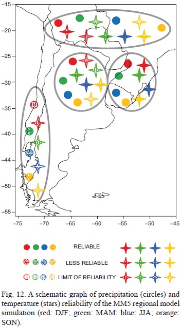

 

5. Summary and conclusions

This work shows the results of the MM5 regional model, driven by the HadAM3H model for the period 1970-1989 over southern South America. This 20-year continuous regional simulation is focused on evaluating the capability of the nested modeling system to represent spatial patterns of seasonal mean climate and its annual cycle of precipitation and temperature over selected subregions. It is important to highlight that the analysis undertaken in this study does not diagnose the physical explanation for model errors, but it may suggest possible pathways for model improvement in future works.

In general, the MM5 regional model is able to represent the spatial distribution of rainfall throughout the year, showing an underestimation of rainfall over subtropical latitudes, south of Brazil, Uruguay, and the center of Argentina and an overestimation over center and southern Chile.

The regional model reproduces the main features of the spatial distribution of surface air temperature adequately. However, there are some systematic bias such as a positive bias in central and northern Argentina and a negative bias in mountainous regions for all seasons. Comparing the spatial distribution of temperature and precipitation biases altogether, it can be concluded that a negative (positive) bias in precipitation is associated with a positive (negative) bias in surface air temperature.

The annual cycle of the simulated precipitation agrees quite well with the annual cycle of the CRU observations in most of the selected regions, except for some overestimation and underestimation.

It is important to highlight that the annual cycle of precipitation over Cuyo and La Plata basin is well represented by the MM5 regional model. Over regions located at the southern tip of the continent the model always overestimates the mean monthly precipitation. Regions located over the center of the model domain show a very satisfactory representation of the annual cycle of precipitation.

The shape of the annual cycle of modeled average temperature is similar to the observed annual cycle for each of the selected regions. Regardless of the subregion, the model shows a positive bias in mean temperature during autumn and a negative bias for spring. However, some exceptions to this behavior can be noted, such as the overestimation of summer temperatures over central Argentina and the underestimation of winter temperatures over southeastern South America.

The model also adequately represents the spatial distribution of rainfall interannual variability compared to CRU observations throughout the domain, as well as the latitudinal displacement of the maximum interannual variability observed in central and southern Chile along the year. However, it has some differences (discussed previously) with respect to modeled and observed intensities.

The MM5 regional model captures the maximum interannual variability of temperature observed during transition seasons, however, larger bias are found for summer and winter. Moreover, regardless of season, the regional model shows a tendency to overestimate the interannual variability of mean temperature.

Overall, the regional model is able to reproduce the general features of regional climate. A survey of the literature reveals that the magnitude of the biases found here is comparable to that of other regional climate simulations for the South American domain (Misra et al., 2003; Giorgi et al., 2004; Solman et al., 2007; Pesquero et al., 2009; among others).

From the evaluation of both variabilities and biases, it can be concluded that the MM5 model simulation is reliable (less reliable) over southern Brazil, Uruguay and the center-east of Argentina (subtropical latitudes and central and southern Chile).

The regional simulation clearly showed added value over the driven global model. It was found that the present simulation reproduces reasonably well the regional climatic features in terms of temperature and precipitation compared to observed datasets. Therefore the current model setup is considered adequate for application in future climate studies for southern South America.

 

Acknowledgments

We would like to thank the Hadley Centre for providing the HadAM3H data. This work was partially supported by UBACYT-Y028, CLAR-IS-LPB (A Europe-South America Network for Climate Change Assessment and Impact Studies in La Plata Basin [http://www.claris-eu.org/]) and CONICET grants PIP 112-201101-00189 and PIP 112-200801-00195.

 

References

Alexandru A., R. de Elía and R. Laprise, 2007. Internal variability in regional climate downscaling at the seasonal scale. Mon. Weather Rev. 13, 3221-3238.         [ Links ]

Alves L. and J. A. Marengo, 2009. Assessment of regional seasonal predictability using the PRECIS regional climate modeling system over South America. Theor. App. Climat. 100, 337-350, doi:10.1007/s00704-009-0165-2.         [ Links ]

Caya D. and S. Biner, 2004. Internal variability of RCM simulations over an annual cycle. Clim. Dynam. 22, 33-46.         [ Links ]

Chen F. and J. Dudhia, 2001. Coupling and advanced land-surface hydrology model with the Penn State-NCAR MM5 modeling system. Part I. Model implementation and sensitivity. Mon. Weather Rev. 129, 569-585.         [ Links ]

Chou S. C., A. Lyra, F. Pesquero, L. M. Alves, G. Sueiro, D. J. Chagas, J. A. Marengo and V. Djurdjevic, 2009. Improvement of long-term integrations by increasing RCM domain size. In: 21st century challenges in regional-scale climate modeling. Proceedings of the Second International Lund RCM Workshop. Lund University, Sweden.         [ Links ]

Chou S. C., J. A. Marengo, A. Lyra, G. Sueiro, J. F. Pesquero, L. Alves, G. Kay, R. Betts, D. Chagas, J. L. Gomez, J. Bustamante and P. Tavares, 2012. Down-scaling of South America present climate driven by 4-member HadCM3 runs. Clim. Dynam. 38, 635-653, doi:10.1007/s00382-011-1002-8.         [ Links ]

Christensen O. B., 1999. Relaxation of soil variables in a regional climate model. Tellus 51A, 674-685.         [ Links ]

Christensen O. B., M. A. Gaertner, J. A, Prego and J. Polcher, 2001. Internal variability of regional climate models. Clim. Dynam. 17, 875-887.         [ Links ]

Da Rocha R. P., C. A. Morales, S. V. Cuadra and T. Ambrizzi, 2009. Precipitation diurnal cycle and summer climatology assessment over South America: an evaluation of Regional Climate Model version 3 simulations. J. Geophys. Res. 114, doi:10.1029/2008JD010212.         [ Links ]

De Elia R., D. Caya, A. Frigon, H. Cote, M. Giguére, D. Paquin, S. Biner, R. Harvey and D. Plummer, 2008. Evaluation of uncertainties in the CRCM-simulated North American climate. Clim. Dyn. 30,113-132.         [ Links ]

De Sales F. and Y. Xue, 2006. Investigation of seasonal prediction of the South American regional climate using the nested model system. J. Geophys. Res. 111, doi:10.1029/2005JD006989.         [ Links ]

Dickinson R., R. Errico, F. Giorgi and G. Bates, 1989. A regional climate model for the western United States. Climatic Change 15, 383-422.         [ Links ]

Fernández J. P. R., S. H. Franchito and V. B. Rao, 2006. Simulation of the summer circulation over South America by two regional climate models. Part I: Mean climatology. Theor. Appl. Climatol. 86, 247-260, doi:10.1007/s00704-005-0212-6.         [ Links ]

Gaertner M. A., O. B. Christensen, J. A. Prego, J. Polcher, C. Gallardo and M. de Castro, 2001. The impact of deforestation in the hidrologycal cycle in the Western Mediterranean: an ensemble study with two regional climate models. Clim. Dynam. 17, 857-873.         [ Links ]

Garrand L., 1983. Some improvements and complements to the infrared emissivity algorithm including a parameterization of the absorption in the continuum region. J. Atmos. Sci. 40, 230-244.         [ Links ]

Giorgi F., 1990. On the simulation of regional climate using a limited area model nested in a general circulation model. J. Climate 3, 941-963.         [ Links ]

Giorgi F. and X. Bi, 2000. A study of internal variability of regional climate model. J. Geophys. Res. 105, 29503-29521.         [ Links ]

Giorgi F., X. Bi and J. S. Pal, 2004. Mean, interannual variability and trends in a regional climate change experiment over Europe. I. Present-day climate (1961-1990). Clim. Dynam. 22, 733-756.         [ Links ]

Grell G. A., 1993. Prognostic evaluation of assumptions used by cumulus parameterizations. Mon. Weather Rev. 12, 764-787.         [ Links ]

Grell G. A., J. Dudhia and D. R. Stauffer, 1993. A description of the fifth-generation Penn System/NCAR Mesoscale Model (MM5). NCAR Tech Note NCAR/ TN -398+1A, 107 pp.         [ Links ]

Grell G. A., L. Schade, R. Knoche, A. Pfeiffer and J. Egger, 2000. Nonhydrostatic climate simulations of precipitation over complex terrain. J. Geophys. Res. 105, 29595- 29608, doi: 10.1029/2000JD900445.         [ Links ]

Hawkins E. and R. Sutton, 2009. The potential to narrow uncertainty in regional climate predictions. Bull. Amer. Meteor. Soc. 90, 1095-1107.         [ Links ]

Hong S. and H. Pan, 1996. Non-local boundary layer vertical diffusion in a medium-range forecast model. Mon. Weather Rev. 124, 2322-2339.         [ Links ]

Hsie E. Y., R. A. Anthes and D. Keyser, 1984. Numerical simulation of frontogenesis in a moist atmosphere. J. Atmos. Sci. 41, 2581-2594.         [ Links ]

Ji Y. and A. D. Vernekar, 1997. Simulation of the Asian summer monsoons of 1987 and 1988 with a regional model nested in a global GCM. J. Climate 10, 1965-1979.         [ Links ]

Kalnay E., M. Kanamitsu, R. Kistler, W. Collins, D. Deaven, L Gandin, M. Iredell, S. Sana, G. White, J. Woollen, Y. Zhu, M. Chelliah, W. Ebisuzaki, W. Higgins, J. Janowiak, K. C. Mo, C. Ropelewski, J. Wang, A. Leetmaa, R. Reynolds, R. Jenne and D. Joseph, 1996. The NCEP/NCAR 40-year reanalysis project. Bull. Amer. Meteor. Soc. 77, 437-471.         [ Links ]

Kitoh A., S. Kusunoki and T. Nakaegawa, 2011. Climate change projections over South America in the late 21st century with the 20 and 60 km mesh Meteorological Research Institute atmospheric general circulation model (MRI-AGCM). J. Geophys. Res. 116, doi:10.1029/2010JD01 4920.         [ Links ]

Kodama Y. M., 1992. Large-scale common features of sub-tropical precipitation zones (the Baiu frontal zone, the SPCZ, and the SACZ). Part I: Characteristics of subtropical frontal zones. J. Meteor. Soc. Japan 70, 813-835.         [ Links ]

Lenters J. L. and K. H. Cook, 1995. Simulation and diagnosis of the regional South American precipitation climatology. J. Climate 8, 2988-3005.         [ Links ]

Lucas-Picher P., D. Caya, R. de Elía and R. Laprise, 2008. Investigation of regional climate models' internal variability with a ten-member ensemble of 10-year simulations over a large domain. Clim. Dynam. 31, 927-940.         [ Links ]

Marengo J. A., T. Ambrizzi, R. P. da Rocha, L. M. Alves, S. V. Cuadra, M. C. Valverde, R. R. Torres, D. C. Santos and S. E. T. Ferraz, 2009a. Future change of climate in South America in the late twenty-first century: Intercomparison of scenarios from three regional climate models. Clim. Dynam., doi:10.1007/s00382-009-0721-6.         [ Links ]

Marengo J. A., R. Jones, L. M. Alves and M. C. Valverde, 2009b. Future change of temperature and precipitation extremes in South America as derived from the PRECIS regional climate modeling system. Int. J. Climatol. 29, 2241-2255.         [ Links ]

Menéndez C. G., M. de Castro, A. Sorensson and J.-P. Boulanger, 2010a. CLARIS project: Towards climate down-scaling in South America. Meteorol. Z. 19, 357-362.         [ Links ]

Menéndez C. G., M. de Castro, J. P. Boulanger, A. D'onofrio, E. Sánchez, A. Sorensson, A. A. Renson, J. Blázquez, A. Elizalde, U. Hansson, H. Le Treut, Z. X. Li, M. N. Nuñez, S. Pfeiffer, N. Pessacg, M. Rojas, P. Samuelsson, S. A. Solman and C. Teich-mann, 2010b. Downscaling extreme month-long anomalies in southern South America. Climatic Change 98, 379-403.         [ Links ]

Misra V., P. A. Dirmeyer, B. P. Kirtman, H.-M. Henry Juang and M. Kanamitsu, 2002. Regional simulation of interannual variability over South America. J. Geo-phys. Res. 107, doi:10.1029/2001JD900216.         [ Links ]

Misra V., P. A. Dirmeyer and B. P. Kirtman, 2003. Dynamic downscalling of seasonal simulations over South America. J. Climate 16, 103-117.         [ Links ]

Mitchell T. D., T. R. Carter, P. D. Jones, M. Hulme and M. News, 2003. A comprehensive set of climate scenarios for Europe and the globe. Working Paper 55. Tyndall Centre for Climate Change Research, Norwich, U.K., 25 pp.         [ Links ]

New M. G., M. Hulme and P. D. Jones, 1999. Representing twentieth-century space-time climate variability. Part I. Development of a 1961-1990 mean monthly terrestrial climatology. J Climate 12, 829-856.         [ Links ]

New M. G., M. Hulme and P. D. Jones, 2000. Representing twentieth-century space-time climate variability. Part II. Development of a 1901-1996 mean monthly terrestrial climatology. J. Climate 13, 2217-2238.         [ Links ]

Nuñez M. N, S. A. Solman and M. F. Cabré, 2008. Regional climate change experiments over Southern South America. II: Climate change scenarios in the late twenty first century. Clim. Dynam. 32, 1081-1095.         [ Links ]

O'Brien T., L. C. Sloan and M. A. Snyder, 2010. Can ensemble of regional climate model simulations improve results from sensitivity studies? Clim Dynam. 37, 1111-1118, doi: 10.1007/S00382-010-0900-5.         [ Links ]

Pesquero J. F., S. C. Chou, C. A. Nobre and J. A. Marengo, 2009. Climate downscalling over South America for 1961-1970 using the Eta Model. Theor. Appl. Climatol, doi:10:/1007/s00704-009-0123-z.         [ Links ]

Pisnichenko I. A. and T. A. Tarasova, 2009. Climate version of the Eta regional forecast model. Evaluating the consistency between the Eta model and HadAM3P global model. Theor. Appl. Climatol, doi:10.1007/s00704-009-0139-4.         [ Links ]

Pope V. D., M. L. Gallani, P. R. Rowntree and R. A. Stratton, 2000. The impact of new physical parame-terizations in the Hadley Centre climate model. Clim. Dynam. 16, 123-146, doi:10.1007/s003820050009.         [ Links ]

Räisänen J., U. Hansson, A. Ullerstig, R. Doscher, L. P. Graham, C. Jones, H. E. M. Meier, P. Samuelsson and U. Willén, 2004. European climate in the late twenty-first century: regional simulations with two driving global models and two forcing scenarios. Clim. Dynam. 22, 13-31.         [ Links ]

Rauscher S. A., A. Seth, J. H. Qian and S. J. Camargo, 2006. Domain choice in an experimental nested modeling prediction system for South America. Theor. App. Climatol., doi:10.1007/s00704-006-0206-z.         [ Links ]

Rayner N. A., D. E. Parker, E. B. Horton, C. K. Folland, L. V. Alexander, D.P. Rowel, E. C. Kent and A. Kaplan, 2003. Global analyses of SST, sea ice, and night marine air temperature since the late nineteenth century. J. Geophys. Res. 108, doi:10.1029/2002JD002670.         [ Links ]

Rinke A. and K. Dethloff, 2000. On the sensitivity of a regional Arctic climate model to initial and boundary conditions. Clim. Res. 14, 101-113.         [ Links ]

Rinke A., K. Dethloff, J. J. Cassano, J. H. Christensen, J. A. Curry, P. Du, E. Girard, J.-E. Haugen, D. Jacob, C. G. Jones, M. Keltzow, R. Laprise, A. H. Lynch, S. Pfeifer, M. C. Serreze, M. J. Shaw, M. Tjernstrom, K. Wyser and M. Zagar, 2006. Evaluation of an ensemble of Arctic regional climate models spatiotemporal fields during the SHEBA year. Clim. Dynam. 26, 459-472, doi:10.1007/s00382-005-0095-3.         [ Links ]

Rojas M. and A. Seth, 2003. Simulations and sensitivity in a nested modeling system for South America. Part II. GCM boundary forcing. J. Climate 16, 2454-2471.         [ Links ]

Rojas M., 2006. Multiply nested regional climate simulation for Southern South America: Sensitivity to model resolution. Mon. Weather Rev. 134, 2208-2223.         [ Links ]

Saulo A. C., M. Nicolini and S. C. Chou, 2000. Model characterization of the South American low-level flow during the 1997-1998 spring-summer season. Clim. Dynam. 16, 867-881.         [ Links ]

Seth A., S. Rauscher, S. Camargo, J.-H. Qian and J. Pal, 2007. RegCM3 regional climatologies for South America using reanalysis and ECHAM global model driving fields. Clim. Dynam. 28, 461-480, doi:10.1007/s00382-006-0191-z.         [ Links ]

Silvestri G., C. Vera, D. Jacob, S. Pfeifer and C. Teichmann, 2009. A high-resolution 43-year atmospheric hindcast for South America generated with the MPI regional model. Clim. Dynam. 32, 693-709, doi:10.1007/s00382-008-0423-5.         [ Links ]

Solman S. A., M. F. Cabré and M. N. Núñez, 2007. Regional climate change experiments over southern South America. I: Present climate. Clim. Dynam. 30, 533-552, doi:10:1007/s00382-007-0304-3.         [ Links ]

Solman S. A. and N. L. Pessacg, 2012a. Regional climate simulations over South America: Sensitivity to model physics and to the treatment of lateral boundary conditions using the MM5 model. Clim. Dynam., doi:10.1007/s00382-011-1049-6.         [ Links ]

Solman S. A. and N. L. Pessacg, 2012b. Evaluating uncertainties in Regional Climate simulations over South America at the seasonal scale. Clim. Dynam., doi:10.1007/s00382-011-1219-6.         [ Links ]

Solman S. A, E. Sánchez, P. Samuelsson, R. da Rocha, L. Li, J. A. Marengo, N. L. Pessacg, R. Remedio, C. Chou, H. Berbery, H. Le Treut, M. de Castro and D. Jacob, 2013. Evaluation of an ensemble of the regional climate models simulations over South America driven by ERA-Interim reanalysis: Model performance and uncertainties. Clim. Dynam., doi:10. 1007/s00382-013-1667-2.         [ Links ]

Sörensson A. A., C. G. Menéndez, P. Samuelsson, U. Willén and U. Hansson, 2010. Soil-precipitation feedbacks during the South American monsoon as simulated by a regional climate model. Climatic Change 98, 429-447, doi:10.1007/s10584-009-9740-x.         [ Links ]

Stephens G. L., 1978. Radiation profiles in extended water clouds. II. Parameterization schemes. J. Atmos. Sci. 35, 2123-2132.         [ Links ]

Stephens G. L., 1984. The parameterization of radiation for numerical weather prediction and climate models. Mon. Weather Rev. 112, 826-867.         [ Links ]

Vanvyve E., N. Hall, C. Messager, S. Leroux and J. P. van Ypersele, 2008. Internal variability in a regional climate model over West Africa. Clim. Dynam. 30, 191-202.         [ Links ]

Vera C., G. Silvestri, B. Liebmann and P. González, 2006. Climate change scenarios for seasonal precipitation in South America from IPCC-AR4 models. Geophys. Res. Lett. 33, L13707,         [ Links ]

Vera C. and G. Silvestri, 2009. Precipitation interannual variability in South America from the WCRP-CMIP3 multi-model dataset. Clim. Dynam. 32, 1003-1014, doi:10.1007/s00382-009-0534-7.         [ Links ]

Von Storch H., 2005. Models of global and regional climate. Meteorology and climatology. In: Encyclopedia of hydrological sciences, vol. 1 (M. G. Anderson, Ed.), Wiley, pp. 478-490.         [ Links ]

Weisse R., H. Heyen, and H. von Storch, 2000. Sensitivity of a regional atmospheric model to a sea state-dependent roughness and the need of ensemble calculations. Mon. Weather Rev. 128, 3631-3642.         [ Links ]