


Servicios Personalizados
Revista
Articulo
 Inglés (pdf)
 Artículo en XML
 Referencias del artículo
 Enviar artículo por email
Indicadores
-
 Citado por SciELO
 -
 Accesos
Links relacionados
-
 Similares en
SciELO
Similares en
SciELO
Compartir

 Permalink
Atmósfera
versión impresa ISSN 0187-6236
Atmósfera vol.27 no.1 Ciudad de México ene. 2014
Synthetic generation of the North Atlantic Oscillation Index
MARITZA LILLIANA ARGANIS-JUÁREZ, RAMÓN DOMÍNGUEZ-MORA and GUADALUPE ESTHER FUENTES-MARILES
Instituto de Ingeniería, Universidad Nacional Autónoma de México, Circuito Escolar s/n, Ciudad Universitaria, 04360 México, D.F. Corresponding author: M. L. Arganis-Juárez; e-mail: MArganisJ@iingen.unam.mx
Received May 25, 2012; accepted November 29, 2013
RESUMEN
En este artículo se compararon registros sintéticos de longitud más larga que los registrados históricamente para el Índice de Oscilación del Atlántico Norte. Los registros sintéticos se obtuvieron utilizando el método de intercambio de años de Grinevich y el método de fragmentos de Svanidze, así como el método de Fiering. Los registros generados se pueden utilizar en modelos de simulación para el análisis a largo plazo del comportamiento de los índices de teleconexión, principalmente relacionados con escenarios de cambio climático.
ABSTRACT
In this article synthetic records of longer duration than the historic records of the North Atlantic Oscillation Index were compared. The synthetic records were obtained using the year interchange method and the Svanidze fragments method, as well as the Fiering method. These records can be used in simulation models for the long-term analysis of the behavior of the teleconnection index, predominantly vis-á-vis climate change scenarios.
Keywords: North Atlantic Oscillation, Svanidze, synthetic generation, Fiering, autocorrelation.
1. Introduction
The teleconnection indices measured by the National Oceanic and Atmospheric Administration (NOAA) identify diverse climatic phenomena that take place on the planet during the different seasons of the year (Rodwell et al., 1999). Particularly, variability in the North Atlantic Oscillation (NAO) Index is directly related with alterations in precipitation and with winter events in different regions of Europe (Parker and Folland, 1988; WMO, 1995; Martin-Vide and Fernández-Belmonte, 2001; Stephenson et al., 2002, 2006). This index, which indicates the variability in atmospheric pressure, has two phases, although in recent years a persistent positive phase has been noted, which has raised some uncertainties regarding the possible effect of climate change (Spokes, 2004). Wunsch (1999) applied autoregressive models AR(1) in an attempt to identify the random nature of the NAO oscillations or its possible relation with climatic changes phenomena. A comparison among reconstruction of the NAO Index from proxy data was made by Schmutz et al. (2000). Cook and D'Ar-rigo (2002) made a multiproxy reconstruction of the NAO Index since A.D. 1400-1979, to research its behavior prior to the twentieth century greenhouse forcing. An analysis about the scaling ranges of its fluctuations upon several delay times trying to identified the NAO Index as a Markov process were made by Collette and Ausloos (2004), who applied historical data from January 1825 to November 2002. Martínez et al. (2010) applied different fractal concepts and dynamic system concepts that pointed to the random nature and need of stochastic models to represent time evolution of the NAO Index. An extensive review of historical studies about the NAO Index can be found in Stephenson et al. (2002).
Caron and O'Brien (1998) conceived a method that successfully reproduces another index, the sea surface temperature (SST) signatures associated with warm and cold events to study the El Niño/Southern Oscillation (ENSO) extremes. They developed algorithms for generating synthetic data using frequency domain analyses, in order to extract information regarding the contribution of different frequency oscillations to the associated variability of the time series. They found that the return period of an extreme ENSO warm event having a maximum SST anomaly magnitude of 2 °C occurs approximately every eight warm events, and concluded that a further use for these synthetic data could be as forcing input in coupled ocean-atmosphere or atmospheric numerical models. The envelope of atmospheric response to various SST anomaly forcings associated with ENSO and other pseudoperiodicities can be understood by combining the work of this study and the current modeling studies of coupled air-sea interaction.
The main mechanisms determining the evolution of the NAO are not completely understood (Bojariu and Gimeno, 2003).
Cañellas et al. (2010) examinated teleconnections between the NAO and the wave climate of the northwestern Mediterranean Sea (NWM). In order to avoid fictitious cross-correlations, data were prewhitened by fitting a p-order autoregressive model. To split the temporal and spatial variability, an empirical orthogonal functions (EOF) encoding technique was applied to residuals before searching for teleconnections. They found the NAO phenomenon contributes to the spatial variability found in the northwestern Mediterranean. When the NAO is in its positive phase there is a reinforcement of the northerly cold and dry air masses from the arctic regions, which generates more severe weather conditions over the NWM.
Chaudhuri et al. (2011) analyzed how the NAO affects the Gulf Stream transport by means of an eddy-resolving model.
In order to simulate long-term climate scenarios it is important to have data of longer duration than the historic records; as a consequence, methods for the synthetic generation of time series that reproduce the statistical characteristics of the historic series turn out to be of particular interest. Almost all traditional methodologies of synthetic generation reproduce statistics such as the mean and standard deviation but have difficulties for other type of parameters such as the coefficient of skew or the coefficient of autocorrelation.
In this work, the Svanidze fragments method (Svanidze, 1980), a modification of it (Domínguez-Mora et al., 2001), as well as the Fiering monthly method (Domínguez-Mora and Carlóz, 1982), were used for the generation of monthly synthetic records for a 1000-year record of the NAO Index. These methodologies have been successfully applied in the case of runoff volumes; thus, the Svanidze method has proven to be very practical and relatively simple in its application, with the advantage over other methodologies (for instance, in relation to the autorregresive moving average [ARMA] models) of not requiring data to be normalized, as well as preserving the autocorrelations (Domínguez-Mora et al., 2001, 2005; Domínguez-Mora and Arganis, 2006; Arganis-Juárez et al., 2008).
2. Methodology
2.1 North Atlantic Oscillation Index
The NAO Index is the difference in pressures that exist between the Azores (at 38° N) and Iceland (at 65° N), which becomes of greatest relevance at winter. It has two phases, one positive, associated to warm and humid events, and one negative. Since 1990 and until a short time after the year 2000, the predominance of the positive phase has been observed, as can be seen on Figs. 1 and 2 (NOAA, 2010; European Environment Agency, 2012).

The rotated principal component analysis (RPCA) used by Barnston and Livezey (1987) isolates the primary patterns of teleconnection for all months and allows time series of the patterns to be built. The standardized anomalies are currently calculated based on the re-analysis of the climatological daily mean and the standard deviation for the period 1950-2000 (NCEP/NCAR Climate Data Assimilation System [CDAS]) run in real time. Because other sources of re-analysis (CDC, NCAR, NCDC) may not have the capacity to provide data in a timely basis, a subset of the current database CDAS is available on the Internet. This subset includes monthly and daily means of many standard pressure-level data and surface fluxquantities (NOAA, 2010).
2.2 Year interchange method (Grinevich)
This method is originally applied to a series of volumes or flows. Let us assume that a reservoir's storage capacity must be obtained from m years of historical records. Through simulation calculations of the reservoir's operation or through comparing distribution curves of flow and demand it is easy to find the storage capacity. However, this is only an approximation and the confidence level of the result is not known. If the record could be extended to a large number of years n (1000, 10 000 years), then with the calculations for the operation of the reservoir an empirical distribution function could be built for the storage capacity and thus the solution to the problem could be found; that is, the storage capacity could be established with a given confidence level. An alternate method to obtain the answer to the problem consists on dividing the series observed in annual hydrographs (with mean monthly discharges) and assign numbers in the order of 1, 2,...,m. Randomly selecting hydrographs from the preceding record, a long hydrological series of longitude n can be generated. Figure 3 presents an illustrative plot of this method (Svanidze, 1980).

The advantages of this method are that it is very simple; assumptions about the univariate or multi-variate distribution functions for the mean annual discharge or the mean monthly discharge are not required; and information about the distribution of flow throughout the year is used in its entirety. Since a great variety of groups of years is obtained for different values of the annual total flow, the stages for the series may be arbitrary, e.g. daily discharges or instantaneous discharges, etc.
The disadvantages of this method are that the structure of correlation between the annual flow volumes is not considered, which decreases the required capacity of the reservoir; drought years and humid years are not grouped subject to regulation by the river but are rather grouped arbitrarily; the shape of the hydrograph is limited only by historic annual hydrographs (m years) alternatives; it provides unreliable results for estimations of minimum or seasonal flows; and when hydrographs are joined discontinuities that do not correspond to the input series can be observed.
One significant disadvantage of this method, which consists in not adding the correlation that exists between annual volumes, can be eliminated in the following manner: The coefficient of serial correlation r1 between the adjacent members d of a series can be determined for different initial dates of the hydrologic year, and the division of the hydrograph of the whole series into annual hydrographs can be done where the dependence is the lowest (r1 = min).
2.3 Svanidze fragments method
The Svanidze fragments method (Svanidze, 1980) accomplishes the generation of synthetic records of a periodical times series with relative simplicity. For this, it is required that the historic record of the series of size n be known, as well as the m periods into which the year is divided (e.g, for monthly divisions m = 12). This method is traditionally applied to data for which the total annual sum can be obtained. Once the sum or the total annual mean has been calculated, the proportion (fragments) of each stage of the year relative to the total annual is obtained, that is:

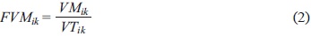
where VTik is the total sum of the measured data for year i of the series k, VMik is the monthly volume for year i of the series k [L3], and FVMk is the fraction (fragment) of the monthly volume relative to the annual total sum VTik. A statistical analysis is performed on the total annual sum to obtain the distribution function of best fit and M synthetic values are randomly determined with that function.
On the other hand, a random selection with or without replacement of the fragments is carried out; these fragments are multiplied by the annual total and thus the M synthetic samples are obtained.
This method can be used with a modification when several time series whose data have a certain degree of cross correlations are available (Arganis-Juárez, 2004).
2.4 Monthly Fiering method
The Fiering method is used to generate monthly runoff records (Domínguez-Mora and Carlóz, 1982).
This method assumes that the next value in the sequence , is equal to the sum of the mean of the month under consideration plus a fraction of the difference of the previous month minus its mean, plus a random component, that is:
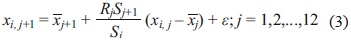
where xi, j is the value corresponding to month j of year i,  is the mean of the historic values of month j, Sj is the standard deviation of the historic values of month j, R is the coefficient of cross correlation between the value of the historic record of months j and and ε is the random component.
The preceding expression can be written as follows, in order for the generated record to have the same monthly and standard deviation values as the historic record:

where tj+1 is a random number with normal distribution of mean zero and standard deviation equal to one.
In order to apply the above expression, the means, variances and coefficients of correlation for each month of the year must be estimated, by following the procedures described in this chapter. Additionally, an initial value is required, so it is suggested to start the method with the first month of the year, and taking the mean as the initial value, generate five years that will not be considered for the study, and then continue with the sequence.
2.5 Annual Fiering method
This method generates an annual time series and calculates the estimated value of variable xi as a function of the annual mean, the coefficient of autocorrelation of order one, the standard deviation and a random number with a standard normal distribution (Domínguez-Mora and Carlóz, 1982):

where xi is the estimated for instant i, y is the mean of the historical series, r1 is the coefficient of autocorrelation of order one, and t1 is the random number with a standard normal distribution (mean of zero and standard deviation of one).
3. Application and results
3.1 Input data
The monthly mean data in ASCII format and standardized with respect to the mean and standard deviation obtained by the CDAS were found on NOAA's webpage, for the period from 1950 to March, 2009. The historic statistics were determined: mean, standard deviation, coefficient of skew and the coefficients of autocorrelation. The lower correlations appear during the months of April and May; this led to the decision to consider yearly periods starting on May of year i and ending on April of year i + 1.
This historical series was used to generate synthetic records with the above-mentioned procedures.
Firstly, the Svanidze fragments method was applied to generate synthetic samples, but its difficulty to reproduce all the statistics was detected; the mean was underestimated in all months, with respect to the historic mean, and the reverse was true for the standard deviation, the coefficient of skew and the coefficient of autocorrelation (overestimation). This was attributed to a combination of the random selection of a year with large fragments (such as years 1962 and 1973) and the random generation of a large annual maximum.
In an attempt to decrease the differences that occurred with this method, the correlations between the annual maximum value of the NAO and the annual mean were determined (Fig. 4).

From Figure 4, a correlation of 0.5587 between the NAO annual maximum and the annual mean is determined; however, it must be realized that this correlation is not completely true, because the NAO annual mean is calculated by taking into account the annual maximum for each year. To eliminate the spurious correlation, the annual mean NAO is normalized by dividing it by the annual maximum value, which leads to the normalized correlation shown in Figure 5, whose value is 0.6079.
Upon analysis of the preceding graphs, three data groups were identified: years with NAO maxima lower than 0.415, years with NAO values between 0.415 and 0.89, and years with values greater than 0.89 (Table I).

A new synthetic generation was performed with the Svanidze generating method. This synthetic generation achieves the random selection of years and fragments by taking into account that if the synthetic NAO annual maximum value is less than 0.415, the selection is done between 1952 and 1953; ifthe NAO synthetic maximum lies between 0.415 and 0.89, inclusive, the selection is done with the years of the second column in Table I; if the maxima exceed 0.89, the selection is done with the remaining years (third column in Table I). Four synthetic series of 1000 record years were determined:
1. Synthetic 1000-year Svanidze fragments series, which uses the Grinevich method with random selection and replacement of the years obtained from the original series and annual maximum. This series is generated assuming a normal distribution.
2. Synthetic 1000-year Svanidze generating series, which uses the Svanidze fragments method with a random selection of the fractions of each month with respect to the historical annual maximum; this selection considers three groups of years, based on the analysis of the correlation between the annual maximum value and the annual mean, and its normalization with respect to the annual maximum. The synthetic annual maxima were determined with the normal distribution function of best fit.
3. Synthetic 1000-year monthly Fiering series.
Graphs for the monthly statistics were created (mean and standard deviation) as well as for the coefficient of skew and the coefficient of autocorrelation, for the three cases under analysis (Figs. 6-9). In all these figures, the first month is May of year i, and the twelfth month is April of year i + 1.
From Figure 6 it can be noticed that the three methods reproduce adequately the average; the standard deviation (Fig. 7) seems to be better reproduced by the Grinevich and Fiering methods, and the skew-ness (Fig. 8) is better reproduced by the Grinevich method. The autocorrelation (Fig. 9) is also well reproduced by all three methods.
Graphs of the distribution functions were created for the synthetic and historical annual maxima and annual means (Figs. 10-15).


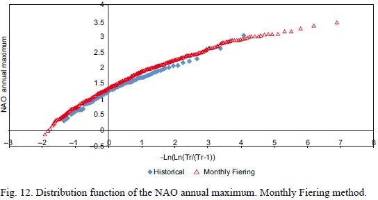


The good agreement between the maxima obtained by the three methods can be seen in Figs. 10-12. However, although we could not obtain values larger than the historical ones with the Grinevich method. In Figs. 13-15 the annual mean was reproduced adequately with the three methods.
4. Conclusions
Synthetic records of longer duration than the historic records for anomalies of the NAO were generated. The procedures that adequately reproduced the historical statistics, as well as autocorrelations, were the year interchange Grinevich method followed by the monthly Fiering method and the Svanidze block-generating method.
The main weakness of the Grinevich method was that NAO scenarios different from the historical ones could not be determined, as can be seen in the distribution functions shown in Figs. 10-13.
The monthly Fiering method allowed us to consider extreme conditions different from historic ones, while preserving the statistics. In particular, the standard deviation and the autocorrelations were reproduced satisfactorily (the maximum differences [MD] in Figs. 7 and 9 were 0.0439 in July and -0.0614 in September, respectively), while the mean was lightly overestimated in the winter months, and the coefficient of skew was also slightly above the historical one in most months; in these cases, the MD were 0.050 in February and -0.8561 in November, respectively.
The Svanidze generating method that uses blocks of years had more difficulty than the monthly Fiering method in reproducing the standard deviation and the coefficient of skew; however, it still preserves the behavior pattern of the mean and of the autocorrelations.
It can be concluded that at least in this case, the best procedure was the monthly Fiering method, which enables the generation of series of longer duration than the historical record for this type of index. The availability of these methodologies is useful for the analysis of different climatic scenarios, which in recent years have become of enormous interest for the scientific community.
5. References
Arganis-Juárez M. L., 2004. Operación óptima de un sistema de presas en cascada para generación hidroeléctrica, tomando en cuenta condiciones reales de operación y el uso de muestras sintéticas para el pronóstico. Ph.D. thesis. Universidad Nacional Autónoma de México, México, 249 pp. [ Links ]
Arganis-Juárez M. L., R. Domínguez-Mora, H. L. Cisneros-Iturbe and G. E. Fuentes-Mariles, 2008. Génération d'échantillons synthétiques des volumes mensuels écoulés de deux barrages utilisant la Méthode de Svanidze Modifiée. Hydrolog. Sci. J. 53,130-141. [ Links ]
Barnston A. G. and R. E. Livezey, 1987. Classification, seasonality and persistence of low frequency atmospheric circulation patterns. Mon. Weather Rev. 115, 1083-1126. [ Links ]
Bojariu R and L. Gimeno, 2003. Predictability and numerical modeling of the North Atlantic Oscillation. Earth-Sci. Rev. 63, 145-168. [ Links ]
Cañellas B., A. Orfila, F. Méndez, A. L. Alvarez and J. Tintoré, 2010. Influence of the NAO on the northwestern Mediterranean wave climate. Sci. Mar. 74, 55-64. [ Links ]
Caron J. M. and J. J. O'Brien, 1998. The generation of synthetic sea surface temperature data for the equatorial Pacific Ocean. Mon. Weather Rev. 126, 2809-2821. [ Links ]
Chaudhuri A. H, A. Gangopadhyay and J. J. Bisagni, 2011. Response of the Gulf Stream transport to characteristic high and low phases of the North Atlantic Oscillation. Ocean Model. 39, 220-232. [ Links ]
Collette C. and M. Ausloos, 2004. Scaling analysis and evolution equation of the North Atlantic Oscillation index fluctuations. Int. J. Mod. Phys. C. 15, 1353-1366. [ Links ]
Cook E. R. and R. D. D'Arrigo, 2002. A well-verified, multiproxy reconstruction of the winter North Atlantic Oscillation Index since A. D. 1400. J. Climate 15, 1754-1764. [ Links ]
Domínguez-Mora R. and G. T. Carlóz, 1982. Análisis estadístico. Manual de diseño de obras civiles, cap. A.1.6. Comisión Federal de Electricidad, México, p. 54. [ Links ]
Domínguez-Mora R., G. E. Fuentes-Mariles and M. L. Arganis-Juárez, 2001. Procedimiento para generar muestras sintéticas de series periódicas mensuales a través del método de Svanidze modificado aplicado a los datos de las presas La Angostura y Malpaso. Series Instituto de Ingeniería, C1-19. [ Links ]
Domínguez-Mora R., C. Cruickshank-Villanueva and M. L. Arganis-Juárez, 2005. Importancia de la generación de muestras sintéticas en el análisis del comportamiento de políticas de operación de presas. Fundación para el Fomento de la Ingeniería del Agua. Ingeniería del Agua 12, 13-25. [ Links ]
Domínguez-Mora R. and M. L. Arganis-Juárez, 2006. Determinación de registros sintéticos de ingresos por cuenca propia de un sistema de presas de la región noroeste de México caracterizada por eventos invernales. Memoirs of the XXII Latin American Hydraulics Congress, Guayana, Venezuela, pp. 1-10. [ Links ]
European Environment Agency, 2012. Available at: [http://www.eea.europa.eu/data-and-maps/find/global#c12=NAO. [ Links ]]
Martín-Vide J. and D. Fernández-Belmonte, 2001. El Indice NAO y la precipitación mensual en la España Peninsular. Investigaciones Geográficas 26, 41-48. Available at: http://www.redalyc.org/pdf/176/17602603.pdf. [ Links ]
Martínez M. D., X. Lana, A. Burgueño and C. Serra, 2010. Predictability of the monthly North Atlantic Oscillation index based on fractal analyses and dynamic system theory. Nonlinear Proc. Geoph. 17, 93-101. [ Links ]
NOAA, 2012. North Atlantic Oscillation (NOA). Available at: http://www.cpc.ncep.noaa.gov/data/teledoc/nao_ts.shtml. [ Links ]
Parker D. E and C. K. Folland, 1988. The nature of climatic variability. Meteorol. Mag. 117, 201-210. [ Links ] Rodwell M. J., D. P. Rowell and C. K. Folland, 1999. Oceanic forcing of the wintertime North Atlantic Oscillation and European climate. Nature 398, 320-323. [ Links ]
Schmutz C., J. Luterbacher, D. Gyalistras, E. Xoplaki and H. Wanner, 2000. Can we trust proxy-based NAO index reconstructions? Geophys. Res. Lett. 27, 1135-1138. [ Links ]
Spokes L., 2004. La Oscilación del Atlántico Norte. Environmental Science Published for Everybody Round the Earth (ESPERE). Available at: http://www.atmosphere.mpg.de/enid/1_Los_oc_anos_y_el_clima/-_La_Oscilaci_n_del_Atl_ntico_Norte_3wa.html. [ Links ]
Stephenson D. B., H. Wanner, S. Broennimann and J. Luterbacher, 2002. The history of scientific research on the North Atlantic Oscillation. In: The North Atlantic Oscillation: climatic significance and environmental impact (J. W. Hurrell, Y. Kushnir, G. Ottersen, M. Visbeck, Eds.). Geoph. Monog. Series 134, 37-50. [ Links ]
Stephenson D. B., V. Pavan, M. Collins, M. M. Junge and R. Quadrelli, 2006. North Atlantic Oscillation response to transient greenhouse gas forcing and the impact on European winter climate: A CMIP2 multi-model assessment. Clim. Dynam. 27, 401-420. [ Links ]
Svanidze, G. G., 1980. Mathematical modeling of hydrologic series. Water Resources Publications, USA, 314 pp. [ Links ]
WMO, 1995. The global climate system review. June 1991-November 1993. World Meteorological Organization, 819 pp. [ Links ]
Wunsch C., 1999. The interpretation of short climate records, with comments on the North Atlantic and Southern Oscillations. B. Am. Meteorol. Soc. 8, 245-255. [ Links ]

