Articles

 

Control of emission rates

 

Y. N. SKIBA and D. PARRA-GUEVARA

Centro de Ciencias de la Atmósfera, Universidad Nacional Autónoma de México, Circuito de la Investigación Científica s/n, Ciudad Universitaria, 04510 México, D.F. Corresponding author: Y. Skiba; e-mail: skiba@unam.mx

 

Received August 28, 2012; accepted February 22, 2013

 

RESUMEN

Se utiliza la ecuación de advección-difusión para describir la dispersión de contaminantes en un área limitada. Se sugieren métodos para prevenir niveles peligrosos de contaminantes en zonas de importancia ecológica. Los métodos se basan en el control de las tasas de emisión de las fuentes y utilizan estimaciones directas y adjuntas de la concentración media de la contaminación en las zonas. Mientras que las estimaciones directas utilizan las soluciones del problema de transporte de un contaminante y permiten llevar a cabo el estudio de la situación ecológica en todo el dominio, las estimaciones adjuntas permiten la obtención de información sólo en las zonas seleccionadas del dominio. Las estimaciones adjuntas se obtienen por medio de soluciones al problema adjunto y dependen explícitamente de las posiciones de las fuentes y sus tasas de emisión, así como de la distribución inicial del contaminante en la región. En cada estimación, la solución al problema adjunto sirve como la función de influencia que muestra la contribución cuantitativa de cada fuente a la contaminación de la zona correspondiente. Por lo tanto, las estimaciones adjuntas constituyen una herramienta muy eficaz en el estudio de la respuesta del modelo a los cambios en las tasas de emisión y las condiciones iniciales, así como en el desarrollo de estrategias de control. Se sugieren varias estrategias de control óptimas y suficientes (no óptimas). Cada estrategia consiste en reducir las tasas de emisión de las fuentes, y define la intensidad máxima admisible (en caso de control óptimo) o una intensidad suficiente (en caso de control suficiente) de cada fuente, para evitar violaciones de las normas sanitarias. En el diseño de dichos criterios se han tomado en cuenta las condiciones dinámicas de la atmósfera o el océano (mar), es decir, los procesos de propagación, dispersión y transformación de contaminantes, así como el número de fuentes que se controlan, sus ubicaciones y las normas sanitarias. Los métodos de control desarrollados se ilustran con ejemplos sencillos, utilizando los modelos de dispersión bidimensionales. Sin embargo, dichos métodos también pueden aplicarse a los modelos tridimensionales. Como ejemplo, en la última parte del artículo, se considera un modelo tridimensional de la dispersión. Además, para ampliar el ámbito de aplicación de los métodos de control de la intensidad de las fuentes, las estrategias de control óptimo se aplican a una fuente que emite una sustancia química para limpiar sistemas acuáticos contaminados con biopelículas (remediación) o petróleo (biorremediación).

 

ABSTRACT

The advection-diffusion equation is used for describing the dispersion of pollutants in a limited area. Methods for preventing dangerous levels of pollutants in ecologically important zones are suggested. The methods are based on the control of emission rates of sources and use the direct and adjoint estimates of the average pollution concentration in the zones. While the direct estimates use solutions of the pollution transport problem and permit to study the ecological situation in the whole domain, the adjoint estimates allow getting information only in the selected zones of the domain. The adjoint estimates are obtained with solutions to the adjoint problem and depend explicitly on the positions of the sources and their emission rates, and on the initial distribution of pollutants in the region. In each such estimate, the adjoint problem solution serves as the influence function that shows the quantitative contribution of every source into the pollution of the corresponding zone. This makes the adjoint estimates very efficient tools in the study of the model response to changes in emission rates and initial conditions, as well as in the development of control strategies. Bothnon-optimal (sufficient) and optimal control strategies are suggested. Each strategy consists in reducing the emission rates of sources, and defines maximum allowable intensity (in case of optimal control), or sufficient intensity (in case of sufficient control) of each source to avoid violations of hygiene standards. Such criteria are designed taking into account dynamic conditions in the atmosphere or ocean (sea), that is, the processes of propagation, dispersion and transformation of pollutants, as well as the number of sources to control, their locations and the sanitary norms. The control methods developed are illustrated with simple examples using two-dimensional dispersion models. However, these methods can also be applied to three-dimensional models. As an example, in the last part of the article, a three-dimensional model of dispersion is considered. In addition, to expand the scope of application of the methods of control of the intensity of sources, the optimal control strategies are applied to a source that emits a chemical substance to clean aquatic systems contaminated with biofilms (remediation) or oil (bioremediation).

Keywords: Dispersion model, adjoint model, control of emission rates of sources.

 

1. Introduction

The main reasons for pollution in any environment are a huge global population and a modern lifestyle that demands and consumes large amounts of goods and services. For example, due to this demand, which has presented a steady increase in recent decades, large volumes of raw materials and fossil fuels are transformed to various pollutants released into the atmosphere (Domenech, 1999; López-Coronado and Guerrero-Nuño, 2004). The environment has mechanisms to dilute and assimilate these pollutants and returning them to nature (Seinfeld, 1992); however, during the last century, anthropogenic activities emit into the atmosphere at short intervals, such large volumes of substances in confined areas (cities, industrial parks, etc.) that the mechanisms of assimilation do not have time to recycle the excess of chemicals and to clean the atmosphere. The result is the accumulation of different primary pollutants, leading to the generation of secondary species (Seinfeld, 1992; Wark et al., 1998; Marinescu et al., 2008), which form a mixture that produces a variety of damages to humans and ecosystems (Caselli, 1996).

A pollutant, depending on its concentration and toxicity, causes various health problems (Kawada, 1984), from respiratory discomfort in healthy people to the increase in mortality among vulnerable populations (cardiac patients, children, elderly persons, etc.). Anyway, pollution is a factor that diminishes the quality of life ofhuman beings. Unfortunately, the impact of mixing of pollutants in ecosystems can be not only local, as in the case of photochemical smog (Bravo et al., 1991), but also regional, as in the acid precipitation (Beilke and Elshout, 1983; Rodhe et al., 1981), or global, as the phenomenon of destruction of the ozone layer and global climate change (Rivera, 1999; Rubinstein, 2001; Karnosky et al., 2003).

Consequently, it is important to design methods for controlling emissions and reducing the concentration of hazardous substances to acceptable health standards (Programma di Ricerca, 2004; Pérez Sesma, 2012). To this end, mathematical models of pollutant dispersion as well as their adjoint models are used (Marchuk and Skiba, 1976; Marchuk, 1986; Panos and Seinfeld, 1986; Skiba, 1997; Davydova-Belitskaya et al., 1999, 2001; Skiba and Parra-Guevara 2000; Parra-Guevara and Skiba 2003, 2006, 2011; Liu et al, 2004, 2005, 2007; Kowalok, 2004; Moreira et al, 2005, 2010; Hinze et al., 2009; Mendoza and García, 2009).

The pollutant dispersion models permit us to carry out the computer-simulation of concentrations of various primary and secondary pollutants in a region (Skiba, 1993, 1997; Skiba and Parra-Guevara, 2000, 2007, 2011; Hussain, 2007; Dorado and Moreira, 2009; Hongfei, 2010; Hongfei and Hongxing, 2011; Parra-Guevara et al., 2010; Fu and Rui, 2011, 2012; Li et al., 2012a), and thereby identify the domains where the emissions have a greater impact. The method allows identifying the main sources of excessive pollution in a selected zone (residential area, park, forest, etc.). In particular, it can be used for the evaluation of pollution levels due to oil spills (Skiba, 1996, 1999; Skiba and Parra-Guevara, 1999; Dang et al, 2012), or to vehicular emissions along the main roads (Skiba and Davydova-Belitskaya, 2003; Chiou and Chen, 2010; Li et al., 2012b; Shafiq and Iqbal, 2012); for estimating parameters which describe the source location and strength (Keats et al., 2007a, b); for the detection of industrial plants which violate the emission rates, prescribed by some control strategy (Skiba, 2003); for the reconstruction of an unknown number of contaminant sources (Yee, 2008); or for the optimal location of a new industrial enterprise, so that its operation will not violate health standards in ecologically most important zones (Marchuk, 1982, 1986; Skiba et al, 2005). The method can also be used to install safety devices in high-risk areas to prevent accidents or unauthorized discharges of contaminants and design emission control strategies for already existing industries (Penenko and Raputa, 1983; Jhih-Shyang, 1998; Parra-Guevara and Skiba, 2000a, b; Zundel and Rentz, 1995; Yan and Zhou, 2008, 2009).

In the present work, an approach based on using dispersion models and corresponding adjoint models is suggested to estimate pollution levels and generate some strategies to control emission rates. These strategies include a restriction of emissions of pollution sources in order to meet sanitary norms. Due to the fact that the sanitary standards represent time averages, the proposed control strategies are aimed at reducing the average concentration of pollutants in a given time interval and region, to an acceptable level. Some control strategies are considered in cases when the dispersion model predicts a violation of sanitary norms.

There are two approaches to monitor and control the emission of pollutants and protect the environment in large industrial regions. The first approach, called "technological path" uses "green" technologies in order to maintain the lowest level of emissions of dangerous pollutants. The second approach consists in establishing various criteria for controlling the emission rates of pollutant sources, and presents a significant mathematical interest.

To illustrate the main mathematical ideas of the control methods, we will often use a simple two-dimensional (vertically integrated) transport model of passive pollutants (i.e. the substances) whose chemical reactions are described by means of a linear law. Of course, all the suggested methods can also be applied to a three-dimensional pollution transport model. On the other hand, the experience gained in the development of such strategies for the atmosphere has allowed expanding the scope of their application (Álvarez-Vázquez et al, 2008, 2010, 2011; Cheng et al., 2007; García-Chan et al., 2009) for cleaning (remediation) aquatic systems polluted by biofilms or petroleum (Parra-Guevara and Skiba, 2007; Skiba and Parra-Guevara, 2011; Parra-Guevara et al., 2011).

 

2. Pollution dispersion model in a limited area

To simplify the study, we will often consider a two-dimensional (vertically averaged) problem of pollutant dispersion. The three-dimensional problem is applied in this work only in the numerical experiment related to the remediation of contaminated aquatic systems. In addition, we will always consider the process of dispersion of contaminants separately from the fluid dynamics problem, supposing that the transport velocity and other dynamic parameters of the problem are known from observations or some dynamic model.

2.1 Boundary and initial conditions

Suppose that in a two-dimensional limited domain D with boundary S, there are N industrial factories located at points r_i = (x_i, y_i), i = 1, 2, N. Let ø(r, t) be a concentration of a pollutant in point r = (x, y) and moment t > 0. To study the propagation of the contaminant in time interval (0, T), we consider in the domain D and time interval (0, T) the advection-diffusion-reaction equation

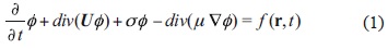
where U(r, t) = {u(r, t), v(r, t)} is the wind velocity vector, σ(r, t) > 0 characterizes the speed of exponential decay of ø(r, t) due to various physical and chemical processes, μ(r, t) > 0 is the turbulent diffusion coefficient, ∇ is the 2D gradient,

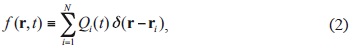
Q_¡(t) is the emission rate of the ith industry, and δ(r-r_i) is the Dirac function. Numerical experiments show that parameterization σø is quite good in the case of such contaminants as CO, SO₂, Pb, C, etc. (Shir and Shich, 1974).

It is assumed that velocity U(r, t) is known from observations or some dynamic model and satisfies the continuity equation

Eq. (1) is solved with the initial condition

Normally the pollution flux through the open boundary S of limited area D is unknown, and the errors made in determining the flux may propagate inside the domain by advection and diffusion, perturbing or destroying the solution. Also, errors in the initial condition (4) and emission rates Q_i(t) can modify the solution. It is therefore important to put such boundary conditions, under which the problem will be posed correctly in a limited area, both physically and mathematically (Marchuk and Skiba, 1976; Marchuk, 1986).

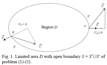
For this purpose, we introduce the projection U_n = U · n of velocity U on the unit external normal n to the boundary S of domain D, and divide the whole boundary into the "inflow" part S (where U_n < 0, and the pollution flux is directed inside D) and "outflow" part S (where U_n ≥ 0, and the pollution flux is directed outside D) (Fig.1). Then we take the following boundary conditions:

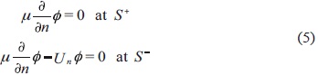
(Marchuk and Skiba, 1976; Skiba, 1997). Skiba and Parra-Guevara (2000, 2011) showed that problem (1)-(5) is well posed according to Hadamard (1923), that is, it has a unique solution that continuously depends on the initial distribution ø⁰(r) and on the number N, emission rates Q_i(t) and positions r _i of the industries.

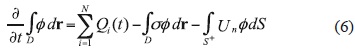
2.2 Equations for the total mass and norm of solution Let us integrate Eq. (1) over domain D and apply conditions (3) and (5). Then we obtain the balance equation for the total mass of pollutant:

One more integral equation is obtained if we multiply Eq. (1) by ø(r, t) and integrate the result over D:

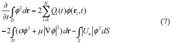
Eqs. (6) and (7) mean that both the total concentration JD ø dr and the solution norm ||ø||=(∫_D ø² dr)^1/2 increase under the influence of non-zero emission rates Q (t), and at the same time decrease due to dissipation (a > 0, yt > 0) and adjective pollution flux through the boundary S of domain D. If ƒ(r, t) = 0 (emission rates are absent), and in addition, there is no dissipation (σ = 0, μ = 0) and U_n = 0 everywhere at boundary S, then both integrals are invariable:

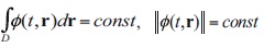
Of course, these conservation laws are valid only under artificial conditions. Nevertheless these two laws and the balance Eqs. (6) and (7) are useful in testing numerical algorithms and computational programs (Skiba, 1997).

2.3 Description of sources in the models

The forcing f(r, t) of Eq. (1) depends on the nature of pollution source. In case of N industrial plants located in D (Fig. 2a), f (r, t) is defined by (2). And if the sources are distributed continuously along the main city roads R_i then

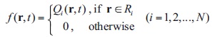
where Q_i(r, t) is the rate of emission of a pollutant along the road R_i, i = 1, 2,..., N (Skiba and Davydova-Belitskaya, 2003). Evidently, a superficially distributed source (e.g. in case of fire) can be described in like manner. However, as it is mentioned in Skiba and Davydova-Belitskaya (2003) and Parra-Guevara and Skiba (2003), the emission rates Q_i(r, t) continuously distributed along some line R (or superficially distributed over some area) can also be described in the discrete form (2) by dividing the line (or area) into small parts and discretizing the function Q_i(r, t) (Fig. 2b). This method was used by Skiba and Davydova-Belitskaya (2003) to introduce in the model the vehicular sources located along the main roads in Guadalajara City. Figure 3 shows the distribution of carbon monoxide concentrations calculated with model (1)-(5) by using the climatic winds of dry season (a) and rainy season (b). One can see the importance of wind direction in the distribution of a pollutant.

 

3. Dual estimates

Figure 3 shows that by solving the problem (1)-(5) we can study the behavior of pollutant concentration in any point of domain D x (0, T). However, this is not an efficient way to answer the important question: To what extent this or that source is responsible for the contamination of a particular zone? It is much easier to answer the question with the adjoint approach, widely used in the model sensitivity study and control theory (Marchuk and Orlov, 1961). The main advantage of this approach is the use of solutions of adjoint problems as valuable information functions (Lewins, 1965).

3.1 Adjoint dispersion model

The adjoint dispersion model in domain D (Fig. 1) and time interval (0, T) is constructed with the help of an operator that is adjoint to the operator of model (1)-(5). The adjoint operator is defined by means of Lagrange identity (Marchuk and Skiba, 1976; Marchuk, 1986), and the adjoint model accepts the form

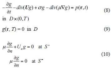
In Eq. (8) the wind velocity U(r, t) and coefficients μ(r, t) and σ(r, t) are the same as in Eq. (1). Let us compare the dispersion problem (1)-(5) with adjoint dispersion problem (8)-(10) in the case when ƒ(r, t) ≡ 0 and p(r, t) ≡ 0. One can see that after using the substitution t'= T - t in Eq. (10), it differs from Eq. (1) only in the sign of velocity U. As a result, the inflow part ST and outflow part of problems (1)-(5) and (8)-(10) are swapped. This fact explains why the boundary conditions (5) are replaced by the conditions (10). It also shows that the adjoint problem is well posed only if it is solved in the opposite time direction: from t = T to t = 0 (Skiba and Parra-Guevara, 2000). That is why we take "initial" condition (9) at the moment t = T.

3.2 Duality principle

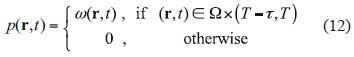
We now show how to define the forcing p(r, t) of the adjoint problem and explain the importance of the adjoint solution g(r, t). Suppose it is required to determine the mean concentration of pollutant ø(r, t) in some ecologically sensible zone Ω⊂D and time interval (T - τ, T). Let co(r, t) be a positive function in domain Ω × (T - τ, T) such that

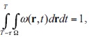
and hence, the integral

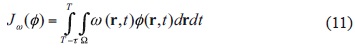
represents an average concentration of pollutant ø (r, t) in space-time domain Ω × (T - t, T).

We now subtract the Eq. (8) pre-multiplied by ø(r, t) from the Eq. (1) pre-multiplied by g(r, t), and integrate the result over domain D × (0, T). The initial and boundary conditions (4)-(5) and (9)-(10) lead then to the duality principle (Marchuk and Skiba, 1976; Skiba and Parra-Guevara, 2011):

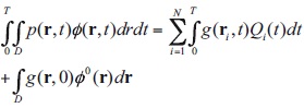
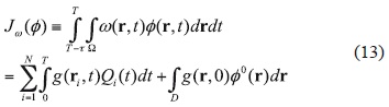
If forcing p(r, t) in (8) is defined as

 

then the last equation leads to one more (equivalent) estimate of average concentration of contaminant ø (r, t) in zone Ω and interval (T - τ, T):

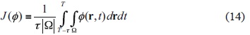
In the particular case that ω(r, t) = 1/(τ |Ω|) in the domain Ω × (T - τ, T), where |Ω| is the area of Ω, estimate (11) leads to the mean concentration of pollutant ø(r, t) in the space-time domain Ω × (T - τ, T):

(the so-called direct estimate). At the same time, Eq. (13) provides the equivalent (dual) adjoint estimate:

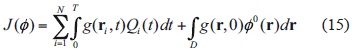
(Marchuk and Skiba, 1976). It means that forcing p(r, t) of adjoint problem (8)-(10) characterizes the average concentration J(ø) of pollutant ø(r, t) in Ω × (T - τ, T). According to adjoint estimate (15), the concentration J(ø) in zone Ω explicitly depends on the emission rates Q_i (t) and initial distribution ø⁰(r) in D, and adjoint solution g(r, t) serves as the weight function that determines the contribution of each source Q_i (t) and initial pollution level ø⁰(r) into the average concentration J(ø) in Ω.

Note that the role of initial distribution of contaminant ø⁰(r) decreases when the interval (0, T - τ) increases (Skiba, 1993). Really, by (12), p(r, t) ≡ 0 in (0, T - t), and, due to the dissipation process (μ > 0, σ > 0), the weight function g(r, 0) in (19) decreases as T - σ increases. If g(r, 0) is relatively small then (15) is reduced to

3.3 Particular qualities of dual estimates

The direct estimate (14) and adjoint estimate (15) are equivalent and complement each other rather well in monitoring the current ecological state. Depending on the situation, one of these formulas may be preferable. The direct estimate (14) uses the solution ø(r, t), and hence, the problem (1)-(5) must be solved again whenever the number N of sources, their positions r_i or emission rates Q_i (t) vary. Of course, the direct evaluation should be used if the pollution concentration is estimated in each point, or in many zones of domain D. However, such comprehensive information is rather costly and often unnecessary. In many cases it is sufficient to know value (14) only in a few ecologically most important zones of region D. Then it is better to find the solutions g_i(r, t) of the adjoint model (8)-(10) for every zone and use the adjoint estimates (15). In some cases the estimates (15) give an immediate solution to non-trivial problems (Skiba et al., 2005; Dang et al, 2012). Also, the adjoint estimates are important to control the emission rates of pollution sources. In contrast to problem (1)-(5), the adjoint problem (8)-(10) is independent of the number of sources N, their positions r_i and emission rates Q_i(t), and therefore its solution can be found for each zone W independently of specific values for all these parameters.

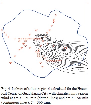
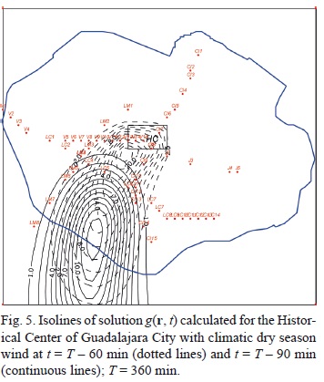
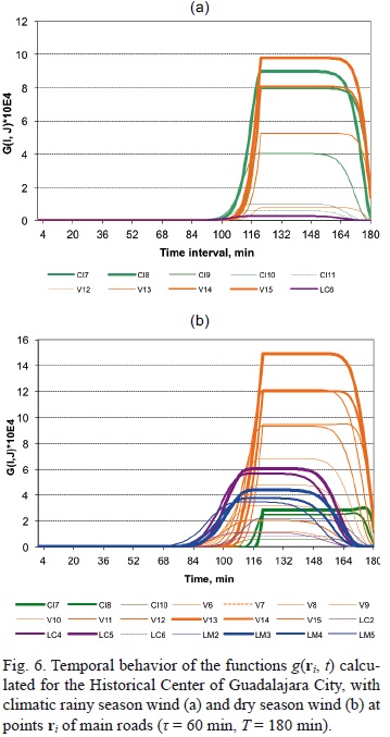
The adjoint method is especially useful when the dispertion problem is considered with time-independent (for example, climatic) parameters U(r), μ(r) and σ(r) (Skiba and Davydova-Belitskaya, 2002). Then any solution to adjoint problem g(r, t), once calculated for a specific zone Ω, can be reused for different parameters N, r_i and Q_i (t) (Figs. 4-6). Moreover, the estimate (16) uses only the values g(r_i, t) in the positions r_i of sources, and therefore, there is no need to keep in a computer the values of adjoint solutions in all grid points.

3.4 Sensitivity of estimates

Suppose that the number K of zones Ω_k ⊂ D (k = 1,...,K is much less than number N of pollution sources. Then the adjoint estimates (15) are very helpful and effective in studying the sensitivity of concentrations J_k(ø) to variations in emission rates Q_i (t), positions r_i and number N of sources, as well as to variations in the initial distribution of contaminant ø⁰ (r).

Let us derive a few sensitivity formulas. Due to the linearity of problem (1)-(5), it is easy to obtain

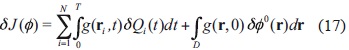
where δJ(ø) is a variation in the mean concentration (15) in zone Ω due to variations in ø⁰ (r), Q_i (t) and/ or N.

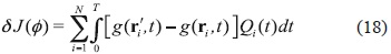
If r_i and r_i are two different positions of sources in domain D then the r_i-dependence of average concentration J(ø) is given by

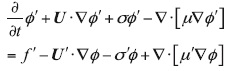
All variations in (17) and (18) are arbitrary. We now obtain a general formula for analyzing the sensitivity of J(ø) with respect to small variations of model parameters. In addition to solution ø to problem (1)-(5), we also consider the solution = ø +ø to perturbed problem

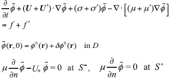
where

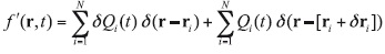
To simplify the study, we assume here that U' and μ' are reduced to zero at the boundary Sand all the perturbations U', ø', μ'‚ σ', δ ø° and δr_i are rather small. Then we can apply the adjoint method to the linearized equation

for perturbations ø' and get

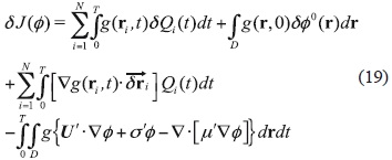
The last two terms of the right-hand side of (19) demonstrate the contribution of small perturbations U', μ', σ', _i to variation SJ(ø) of mean concentration J(ø) in zone Ω. It should be noted that in contrast to estimates (17) and (18), the last term in (19) already contains the solution ø(r, t) of non-perturbed problem (1)-(5). Thus, solution ø(r, t) is not used only if U' = o' = u' = 0 everywhere in D. Then only the adjoint problem (8)-(10) must be solved.

 

4. Three simple strategies for pollution control

Let us formulate the problem of control of emission rates. Suppose that we have a model M that predicts the dispersion of a pollutant ø in a limited area D⊂ R^m (m = 2, 3) and time interval (0, T):

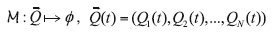
where Q_i (t) ≥ 0 is the rate of emission of contaminant ø of the ith source located at r_i , ∈ D (i = 1, 2,..., N). In particular, (1)-(5) can be taken as such a model. Let the functional (14) be used as the mean concentration J(ø) of pollutant ø in a zone Ω⊂D and time interval [T - τ, T], and let J₀ be a sanitary norm admissible for the pollutant ø. If the model M gives an unfavorable forecast of air quality, that is, the mean concentration exceeds the sanitary norm: J(ø) > J₀, then the emission rates (t) were excessive, and must be reduced in interval (0, T). The idea is to determine such reduced values (t) ≤ (t) in order to prevent high levels of pollutant ø in time-space domain Ω × [T - τ, T]. It means that the re-forecast with the reduced emission rates (t) will give the satisfactory result: J(ø) ≤ J₀.

This inverse problem may have many solutions or none, depending on the initial distribution of pollutant ø⁰(r) in domain D (Parra-Guevara and Skiba, 2003, 2006). So it is an ill-posed problem. In order to get a well-posed problem, one should apply a regularization method that in a sense represents a control strategy. Let us consider three simple examples.

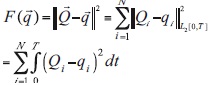
4.1 Strategy 1: Control of total mass of emitted pollutant

This control strategy can be defined as the following optimization problem:

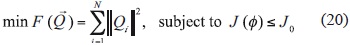
where 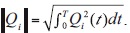Thus, F() represents the total mass of pollutant ø emitted within interval [0, T] by N sources located at points r_i with emission rates Q_i(t). The solution of problem (20) is

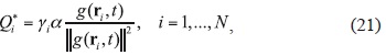
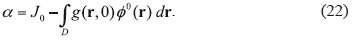
(Parra-Guevara and Skiba, 2000a; Parra-Guevara, 2001) where is the quota of the total mass of pollutant, emitted by the ith source when it works at full capacity (i = 1,..., N), and

4.2 Strategy 2: Control of temporal behavior of emission rates

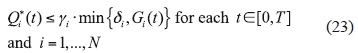
It should be noted that the control strategy (21) has the disadvantage that it may require stopping the sources for some time for the reason that the emission rates are proportional to the adjoint function g(r_i, t), which can be equal to zero. Let us consider a new strategy of control that limits the behavior of emission rates in (0, T), but does not require stopping the activity of sources when the adjoint solution g(r_i, t) reduces to zero.

Again, we should find such Q_i* ∈ L₂(0, T) that J(ø) ≤ J₀. The idea is that intensity Q_i*(t) of the ith source may be high while g(r_i, t) is small, and Q_i*(t) must be low while g(r_i, t) is large. The advantage of this approach is that, in some periods of time (for example, when g(r_i, t) = 0), the corresponding source will be allowed to operate at full capacity (Parra-Guevara and Skiba, 2000a, 2003; Parra-Guevara, 2001). Let us define auxiliary functions

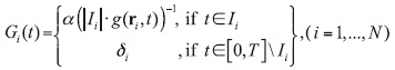
where I_i ={t∈[0,T]|g(r_i,t)>o} and|I_i|denotes its longitude, δ_i is the maximum emission rate corresponding to the ith source, and [0, T]\ I_i is the complement of set I_i to set [0, T]. Then the solution is

4.3 Strategy 3: Optimal time-independent emission rates

Suppose that Q_i is the maximum possible emission rate of ith source located at r_i and

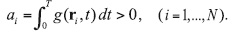
Assume that all sources operate at full capacity power that results in the violation of the sanitary norm: J(ø) > J₀ (and (15) and (22), this means that To prevent the excessive pollution of the zone, some emission rates must be reduced. We now find the maximum possible time-invariant emission rates Q_i* ≤ Q_i which minimize the values Q_i - Q_i*, do not lead to violation of the sanitary norm, giving the optimal result: J(ø ) = J0, that is,

Let us reformulate this strategy as the optimization problem

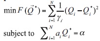
With Lagrange multipliers we obtain

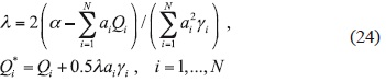
(Parra-Guevara and Skiba, 2000a; Parra-Guevara, 2001). Obviously, Q_i* ≤ Q_i, for all i, since λ < 0, besides Q_i* ≈ Q_i for small γ_i. Thus, this control results in limiting the emissions from the sources for which the corresponding values a_i are large.

 

5. General strategy of optimal control

be a functional defined in the domain

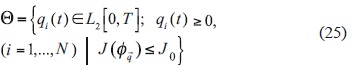
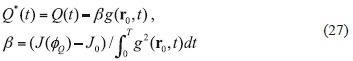
Thus Θ is the set of such emission rates q(t) that guarantee the compliance with the sanitary standard in a zone Ω: J(ø) ≤ J₀. The optimal control consists in finding such rates Q* (t)∈Θ that minimize the functional F(a) in Θ:

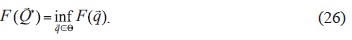
(Parra-Guevara and Skiba, 2000a; Parra-Guevara, 2001; Skiba and Parra-Guevara, 2011). Clearly, the control depends on the norm ||·|| used, and (t) is the optimal solution that represents the least restriction on the sources. This variational problem is generally solved with an iterative optimization method using successive evaluation of the dynamic model M (Elbern and Schmidt, 1999; Robertson and Langer, 1998). As a general rule, this process is not very efficient because it requires many calculations due to the complexity of model M. Therefore we will now describe another method based on using the adjoint operator and adjoint model, which allows us to solve the problem of optimal control without consistent estimation of model M.

Note that the solution of problem (26) depends critically on the parameter a defined by (22). Indeed, for a < 0 there is no solution to (26) because the standard of health does not hold even if all emissions are reduced to zero (that is, any production activity is stopped). The following three results in this section were proved in Parra-Guevara and Skiba (2006, 2007).

Theorem 1

Let α = 0. Then the optimal control problem (26) has only one solution:

Theorem 2

If α > 0 then the optimal control problem (26) has the unique solution (t)∈Θ such that Q_i*(t) ≤ Q_i(t)(0 ≤ t ≤ T, 1 ≤ i ≤ N) and J(ø) = J₀.

If there is only one source, the statement of Theorem 2 can be refined:

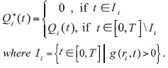
Theorem 3

Suppose that there is only one source with emission rate Q(t) located at the point r₀. If a > 0 and J(ø) > J₀ then

is the only solution for the problem of optimal control (26), on condition that it is a nonnegative function in [0, T].

In connection with Theorem 2, the set of potential solutions (25) is reduced to

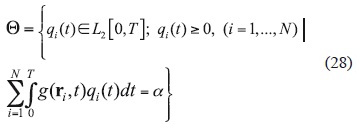
An approximate (numerical) solution to the problem of optimal control can be obtained with highly effective numerical algorithm of sequential orthogonal projections (Parra-Guevara and Skiba, 2006). From the computational viewpoint, the new set (28) is much smaller than (25), and therefore preferable in calculations.

5.1 Strategies of control based on convex linear combinations

A new strategy to control emissions can always be developed with a convex linear combination of the existing strategies. Let K be a number of previously defined control strategies, besides, each strategy ensures compliance with the health standard in a zone Ω: J(ø) ≤ J₀. Let ξ₁, ξ₂,..., ξ_K be positive constants such that ξ₁ + ξ₂ + ... + ξ_K = 1 , and let Q*_{i k} be a sufficient (or optimal) emission rate found by means of the kth control strategy for the ith source (i = 1,..., N,k = 1,...,K). Then the emission rates

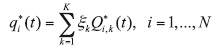
represent a new sufficient (non-optimal) strategy that also guarantees compliance with the health standard in the zone Ω: J(ø) ≤ J₀.

 

6. Control of the source that emits lead particles

To illustrate the developed methods we now consider two examples in which the source emits the lead particles.

Example 1. Let D = (0, 2 km)x(0, 2 km) be a square domain, while the single point source, located at r₀ = (1.8, 0.2), emits lead particles with emission rate Q = 3.8 kg/h. For simplicity, we neglect the initial distribution of lead: ø⁰(r) = 0 in D. The coefficients of deposition and diffusion are σ = 0.001 h^-1 and μ = 0.04 km²h^_1, respectively. The non-divergent wind velocity U = (u, v) is defined by the stream function ψ = xy:

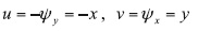
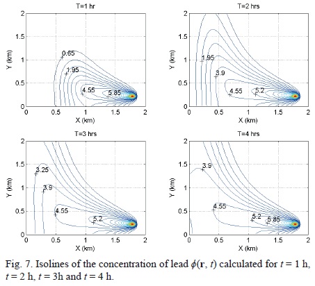
The dispersion model (1)-(5) and adjoint model (8)-(10) are considered in the four-hour interval (0, T). We will monitor the mean lead concentration J(ø) in the zone Ω = [0, 0.5]x[0.5, 1.0] during the whole interval (0, T), that is (τ = 4 h). The sanitary norm is J₀ = 1.5 μg m^-3 (Seinfeld, 1992).

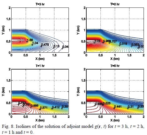
Isolines of the concentration of lead at intervals of one hour are presented in Figure 7, while isolines of the solution g(r, t) of adjoint model (8)-(10) are given in Figure 8. Figure 7 shows a clear increase in the concentration of lead when the direction of the wind is changed from southeast to northwest. Figure 8 demonstrates that during the four-hour interval (from t = 4 to t = 0), the step function p(r, t) shifts in the direction of vector -U (that is, from north-west to south-east), as it should. The mean concentration of lead J(ø ) calculated in zone Ω with emission rate Q is 2.11 mg m^-3. The result is unsatisfactory (J(ø) > J₀), and we will apply and compare five different control strategies: the control strategies (21), (23) and (24) with emission rates Q* (i = 1, 2, 3) and two control strategies defined with the convex linear combinations Q₄* = 0.3 · Q*_i + 0.7 · Q₃* and Q₅* = 0.5 · Q₂* + 0.5 · Q₃*.

The mean lead concentrations obtained in zone Ω when the model (1)-(5) is solved with emission rates Q₁*(t), prescribed by the five control strategies (i = 1,..., 5), are shown in Table I, while Figure 9 shows the temporal behavior of Q₁*(t).

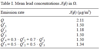
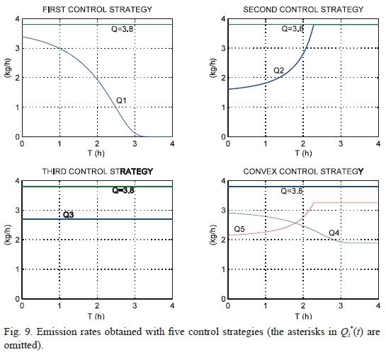
All five control strategies correspond to the level of health, and provide an alternative to the original source intensity Q. However, the emission rate Q₃* (optimal control), as well as the rates Q₄* and Q₅* (convex control) are the most preferred as they require less drastic changes in the intensity of the original source. Although the emission rate Q₂* is only 40% of the original rate Q in the first half of the time, it coincides with the original rate Q during the second half of the time, and this fact can also be attractive.

Note that, like the original rate Q, the optimal emission rate Q₃ is stationary (it is 71% of Q). This makes Q₃ a simple alternative to the original industrial source activity. The results show that among the five strategies, the first strategy with emission rate Q₁ has the most serious consequences for the industrial plant activity, because it requires the work stoppage during 25% of the total time.

Example 2. In this example domain D and wind velocity U are the same as in Example 1. Moreover, the source also emits lead particles and is located at the same place. However, we now consider the four different original emission rates of the source:

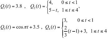
Thus, rate Q₁ is constant, rate Q₂ is invariable during the first hour and then linearly decreases, rate Q₃ is a periodic function with a two-hour period, and rate Q₄ is invariable during the first hour and then linearly increases. The mean lead concentrations J_i(ø) calculated in zone Ω with each emission rate Q_i (i = 1,..., 4) are 2.11 μg m^-3, 2.02 ug m^-3, 1.97 μg m^-3 and 1.81 μg m^-3, respectively. In other words, all the results are unsatisfactory (J_i(ø) > J₀ for any i, where J₀ = 1.5 μg m^-3). In order to prevent the violation of sanitary standards, we apply in all four cases the optimal control method (27). Figure 10 shows both the original emission rates Q₁(t) and the optimal emission rates g_opti(t) given by the control. As it should be, for each i, the mean lead concentration J_i(ø) obtained with the optimal emission rate q_opti(t) coincides with norm J₀ = 1.5 μg m^-3.

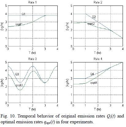
In complete agreement with the theory, q_opti(t) ≤ Q_i(t) for all t ∈ (0.4) and 1 ≤ i ≤ 4. Moreover, Figure 10 shows that for each i, q_opti(t) = Q_i(t) during the last hour (3 ≤ t ≤ 4). It means that the optimal and original emission rates coincide to each other during the time interval when the value g(r₁, t) of the adjoint model solution is equal to zero, and due to (15), the source emissions do not contribute to the pollution of zone Ω. At last, it is interesting to note that in the interval 0 ≤t < 3, in which these values do not match, the temporal behavior of the optimal emission rate q_opti(t) is similar to the time behavior of the corresponding original rate Q,(t) (i = 1,..., 4). This result is useful because it means that the optimal strategy (27) does not require radical changes in the operation of an industrial enterprise.

 

7. Cleaning of polluted aquatic zones

The above-mentioned control methods have been illustrated with simple examples using two-dimensional dispersion models. However, these methods can also be applied to three-dimensional dispersion models. We will consider now a three-dimensional dispersion model for expanding the application scope of pollution control methods to the cleaning of some aquatic zones contaminated with biofilm (remediation) or oil (bioremediation). In these problems, the discharge rate of a source that emits a chemical substance to clean water is controlled.

7.1 Dispersion model

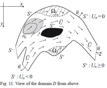
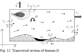
The concentration of a chemical substance (hereinafter the cleaner) ø(r, t) ≡ ø(x,y, z, t) in a domain D⊂R³ (Fig. 11) and time interval (0, T) is estimated with a 3D dispersion model (Skiba and Parra-Guevara, 2011):

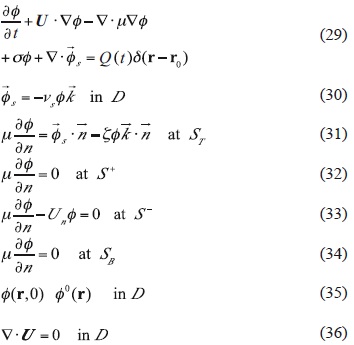
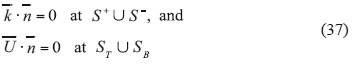
Here U ≡(r,t) is the current velocity that satisfies the continuity equation (36), and μ(r, t) is the turbulent diffusion coefficient. In (29), the term σø parameterizes the decay of a cleaner in the water due to various physical and chemical processes, term ∇ · describes the process of sedimentation of the cleaner with constant velocity v_s > 0, and δ(r- r₀) is the Dirac delta centered in the point of discharge of cleaner r₀. Eq. (31) is the boundary condition at free surface S_T, where coefficient ξ(r, t) characterizes the process of evaporation of cleaner, and (34) represents the boundary condition at bottom S_B of domain D. The boundary conditions (32) and (33) at the lateral surface are identical to conditions (5), and (35) represents the initial distribution of the cleaner at t = 0. Note that ñ is the unit outer normal to the boundary ∂D = S_T U S+ U S^- U S_B of domain D, and = (0,0, 1)^T is the unit vector directed upwards in the Cartesian coordinate system, besides,

Also note that conditions (31)-(34) take into account the topography and free surface of arbitrary form.

It is shown in Skiba and Parra-Guevara (2011) that the three-dimensional problem (29)-(36) is well posed, that is, its solution exists, is unique and stable to perturbations in forcing and initial condition

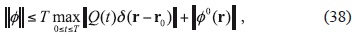
and satisfies the mass balance equation

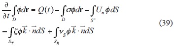
Since 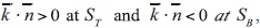the total mass of the cleaner increases due to the discharge rate Q(t) and decreases due to the chemical transformation, advective flow through S+, evaporation and sedimentation.

7.2 Optimal control of discharge rates

Assume now that there are N polluted zones Ω_i (i = 1,..., N) in an aquatic system (domain D), and we should purify them with the help of a chemical agent (Parra-Guevara and Skiba, 2007). Being released at a point r₀ ∈D (Fig.12), the chemical substance spreads due to advection and diffusion, and while reaching the zones Ω_i, purifies polluted water. The goal is to find an optimal position of the source r₀, in sense that the emission of the cleaning agent in such a point will minimize its consumption (that is, will generate in the zones Ω, the minimum concentrations of the cleaning agent necessary for water purification). In a case where the contaminant is fairly stable (biofilm), the critical concentration of an antimicrobial agent (chlorine, iodine, etc.) must be maintained in each zone Ω_i for a long time interval (T - τ, T).

In other words, we have to determine the discharge point r₀ and the emission rate Q , which meet the following constraints:

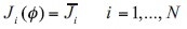
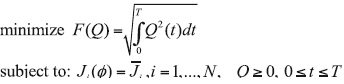
where ø(r, t) is the concentration of a chemical agent determined by the model (29)-(36) with the initial condition ø⁰(r) = 0, and J_i(ø) is its mean concentration (14) in Ω_i. Furthermore, not to damage the ecology of the environment, one should minimize the total mass F(Q) of the chemical agent discharged into the water. In this connection, the optimal control problem is posed as follows:

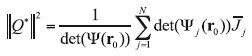
The analytical and numerical solutions of this problem were obtained in Parra-Guevara and Skiba (2011):

 

where Ψ = {Ψ_ij} is the Gram matrix of order N whose entries

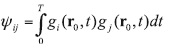
are the inner products of adjoint functions, and matrix Ψ_i, is obtained from Ψ by replacing its ith column with the corresponding components of the vector of critical concentrations 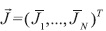. Then the optimal discharge point r₀ is found while minimizing the functional.

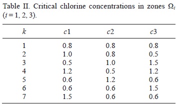
Example 3. With the aim to demonstrate the skill of the method, we now consider a simple example of remediation in a three-dimensional channel 120 m long [0, 120], 10 m wide [0, 10], and 4 m deep [0, 4], H = 4. The following three zones Ω contaminated by biofilms (N = 3) are considered:

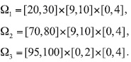
The critical concentrations of the cleaning agent c_i (gm^-3) in the zones vary from one experiment to another (Table II) and generate different optimal discharge rates Q_k* (Fig. 13). The parameters of the three-dimensional adjoint model are taken as follows: the velocity vector is horizontally directed along the channel and is equal to 30 mh^-1, μ = 6 m²h^_1, a = 1 h^-1 and the processes of evaporation and sedimentation are neglected. The cleaner (chlorine) is discharged at the point r₀ = (3, 2.2, 2) during the total time interval of 4 h: (0, T) ≡ (0, 4), and the mean concentration is controlled within the last one-hour interval (3, 4), i.e., τ = 1 h.

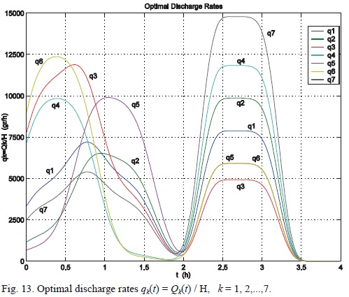
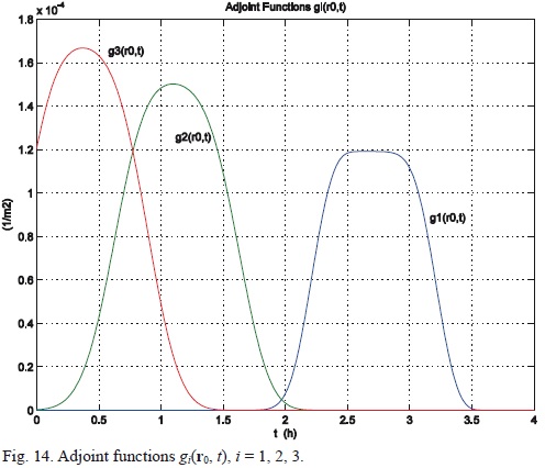
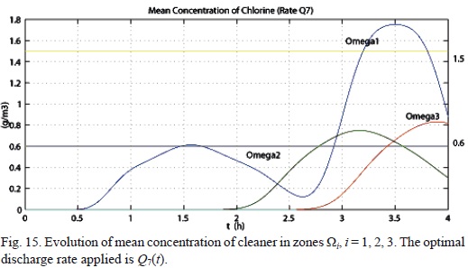
The adjoint functions g_i(r₀, t) for the three zones (i = 1, 2, 3) are given in Figure 14. For the 7th experiment, the evolution of mean chlorine concentration in zones Ω_i (i = 1, 2, 3) is shown in Figure 15, while isolines of the mean chlorine concentration in  domain D at the final moment T = 4 h are presented in Figure 16. The optimal discharge rate applied is Q₇(t). In all experiments, the optimal discharge rate was successfully found with (40).

 

8. Conclusions

In this work, the fluid dynamics is assumed to be known, and the problem of dispersion of contaminants, governed by the advection-diffusion equation, is considered separately from the fluid dynamics. A few methods are suggested for estimating the mean concentration of pollutants in ecologically sensitive zones and preventing their dangerous levels through a control of emission rates of sources. The methods use the adjoint approach and equivalent direct and adjoint estimates of pollution concentration in specific zones. We use the fact that the adjoint estimates depend explicitly on the number, positions and emission rates of the sources and the initial distribution of pollutants in the region, and the solutions of adjoint problems serve in such estimates as weight function providing valuable information on the contribution of each source and initial data into the pollution of the zone. These properties make the adjoint estimates efficient for studying the model response to variations in the emission rates and initial conditions, and for developing control strategies.

Both non-optimal (sufficient) and optimal control strategies have been developed. The objective of each control strategy consists in preventing the violation of existing sanitary standards by means of reducing the emission rates of sources. Each control strategy is designed by using the pollution dispersion model, its adjoint model, and taking into account the number of sources to control, their locations, initial distribution of pollutant in the domain, and corresponding sanitary standards. The methods are illustrated by simple examples. The methods developed for the air-quality control are also applied for cleaning a few aquatic zones polluted with biofilm (remediation) or oil (bioremediation).

 

Acknowledgements

The authors are grateful to Dr. V. Davydova-Belitskaya for providing some figures. This work was partially supported by the projects PAPIIT IN104811-3 and PAPIIT IN103313-2 (UNAM, México) and by the grants 14539 and 25170 of Sistema Nacional de Investigadores (Conacyt, Mexico).

 

References

Álvarez-Vázquez L. J., A. Martínez, M. E. Vázquez-Méndez and M. A. Vilar, 2008. Vertical slot fishways: Mathematical modeling and optimal management. J. Comput. Appl. Math. 218, 395-403.         [ Links ]

Álvarez-Vázquez L. J., N. García-Chan, A. Martínez, M. E. Vázquez-Méndez and M. A. Vilar, 2010. Optimal control in wastewater management: a multi-objective study. Communications in Applied and Industrial Mathematics 1, 62-77.         [ Links ]

Álvarez-Vázquez L. J., N. García-Chan, A. Martínez, and M. E. Vázquez-Méndez, 2011. SOS: A numerical simulation toolbox for decision support related to wastewater discharges and their environmental impact. Environ. Modell. Softw. 26, 543-545.         [ Links ]

Beilke S. and A. J. Elshout (Eds.), 1983. Acid deposition. Proceedings of the CEC workshop, Berlin, 9 September 1982. D. Reidel Publishing Company, Boston, 235 pp.         [ Links ]

Bravo A. H., R. Sosa and R. Torres, 1991. Ozono y lluvia ácida en la ciudad de México. Ciencias 22, 33-40.         [ Links ]

Caselli M., 1996. La contaminación atmosférica. Siglo XXI, Mexico, 193 pp.         [ Links ]

Cheng S. Y., J. B. Li, B. Feng, Y. Q. Jin and R. X. Hao, 2007. A Gaussian-box modeling approach for urban air quality management in a Northern Chinese City -II. Pollutant emission abatement. Water Air Soil Poll. 178, 15-36.         [ Links ]

Chiou Y. C. and T. C. Chen, 2010. Direct and indirect factors affecting emissions of cars and motorcycles in Taiwan. Transportmetrica 6, 215-233.         [ Links ]

Dang Q. A., M. Ehrhardt, G. L. Tran and D. Le, 2012. Mathematical modeling and numerical algorithms for simulation of oil pollution. Environ. Model. Assess. 17, 275-288.         [ Links ]

Davydova-Belitskaya V., Y. N. Skiba, S. N. Bulgakov and A. Martínez, 1999. Modelación matemática de los niveles de contaminación en la ciudad de Guadalajara, Jalisco, México. Parte I. Microclima y monitoreo de la contaminación. Rev. Int. Contam. Ambie. 15, 103-111.         [ Links ]

Davydova-Belitskaya V., Y. N. Skiba, A. Martínez and S. N. Bulgakov, 2001. Modelación matemática de los niveles de contaminación en la ciudad de Guadalajara, Jalisco, Mexico. Parte II. Modelo numérico de transporte de contaminantes y su adjunto. Rev. Int. Contam. Ambie. 17, 97-107.         [ Links ]

Domenech X., 1999. Química de la contaminación. Miraguano, Madrid, 160 pp.         [ Links ]

Dorado R. M. and D. M. Moreira, 2009. Contaminant dispersion simulation with micro-meteorological parameters generated by LES in the area around the Angra nuclear power plant. Proceedings of the International Nuclear Atlantic Conference. Associacáo Brasileira de Energia Nuclear, Rio de Janeiro, Brazil, 11 pp.         [ Links ]

Elbern H. and H. Schmidt, 1999. A four-dimensional variational chemistry data assimilation scheme for Eulerian chemistry transport modeling, J. Geophys. Res. 104, 18583-18598.         [ Links ]

Fu H., 2010. A characteristic finite element method for optimal control problems governed by convection-diffusion equations. J. Comput. Appl. Math. 235, 825-836.         [ Links ]

Fu H. and H. Rui, 2011. A characteristic-mixed finite element method for time-dependent convection-diffusion optimal control problem. Appl. Math. Comput. 218, 3430-3440.         [ Links ]

Fu H. and H. Rui, 2012. A mass-conservative characteristic FE scheme for optimal control problems governed by convection-diffusion equations. Comput. Method. Appl. M. 241-244, 82-92.         [ Links ]

García-Chan N., R. Muñoz-Sola and M. E. Vázquez-Méndez, 2009. Nash equilibrium for a multiobjective control problem related to wastewater management. ESAIMContr. Op. Ca. Va. 15, 117-138.         [ Links ]

Hadamard J., 1923. Lectures on Cauchy's problem in linear partial differential equations. Yale University Press, 316 pp.         [ Links ]

Hinze M., N. N. Yan and Z. J. Zhou, 2009. Variational discretization for optimal control governed by convection dominated diffusion equations. J. Comput. Math. 27, 237-253.         [ Links ]

Hussain J., 2007. Nonlinear models for the effect of pollutants on pollution with time-delay. In: PAMM special issue: Proceedings of the 6th International Congress on Industrial Applied Mathematics (ICI-AM07) and GAMM Annual Meeting, Zürich. Proc. Appl. Math. Mech. 7, 2120029-2120030, doi: 10.1002/pamm.200701011.         [ Links ]

Jhih-Shyang S., 1998. An optimization model for photochemical air pollution control. Eur. J. Oper. Res. 106, 1-14.         [ Links ]

Karnosky D. F., K. E. Percy, R. C. Thakur and R. E. Honrath, 2003. Air pollution and global change: A double challenge to forest ecosystems. In: Developments in environmental science, vol. 3. Air Pollution, global change and forests in the new millenium. (D. F. Kar-nosky, K. E. Percy, A. H. Chappelka, C. Simpson and J. Pikkarainen, Eds.). Elsevier, pp. 1-41.         [ Links ]

Kawada J., 1984. Health effects of air pollutants and their management. Atmos. Environ. 18, 613-620.         [ Links ]

Keats A., E. Yee and F. S. Lien, 2007a. Bayesian inference for source determination with applications to a complex urban environment, Atmos. Environ. 41, 465-479.         [ Links ]

Keats A., E. Yee and F. S. Lien, 2007b. Efficiently characterizing the origin and decay rate of a nonconservative scalar using probability theory. Ecol. Model. 205, 437-452.         [ Links ]

Kowalok M. E., 2004. Adjoint methods for external beam inverse treatment planning. Ph. D. Thesis, University of Wisconsin-Madison, Department of Medical Physics, Madison, Wisconsin.         [ Links ]

Lewins J., 1965. Importance, the adjoint function. Perga-mon Press, Oxford, 172 pp.         [ Links ]

Li L., S. Liu and H. Xu, 2012a. Analysis and thinking of the current condition for traffic pollution of urban roads. Appl. Mech. Mater. 178-181, 859-863.         [ Links ]

Li Y., M. Dong, X. Xiang, Z. Xiang and Y. Pang, 2012b. An optimal control model and the computer algorithm for the diffusion parameter of the drug releasing in the spherical device. Information Technology Journal 11, 1032-1039.         [ Links ]

Liu F., Y. H. Zhang, F. Hu, S. Huang and H. Chen, 2004. Adjoint approach for assessment of chemical risk. Proceedings of the 2004 International Symposium on Safety Science and Technology. Prog. Safety Sci. Tech. 4, 2357-2362.         [ Links ]

Liu F., Y. H. Zhang and F. Hu, 2005. Adjoint method for assessment and reduction of chemical risk in open spaces. Environ. Model. Assess. 10, 331-339.         [ Links ]

Liu F., J. Zhu, F. Hu and Y. Zhang, 2007. An optimal weather condition dependent approach for emission planning in urban areas. Environ. Model. Softw. 22, 548-557.         [ Links ]

López-Coronado G. A. and J. J. Guerrero-Nuño (Eds.), 2004. Ecología urbana en la zona metropolitana de Guadalajara. Editorial Ágata, Guadalajara, Jalisco, 337 pp.         [ Links ]

Marchuk G. I. and V V. Orlov, 1961. On the theory of adjoint functions. In: Neutron physics. Gosatomizdat, Moscow, pp. 30-45.         [ Links ]

Marchuk G. I. and Y. N. Skiba, 1976. Numerical calculation of the conjugate problem for a model of the thermal interaction of the atmosphere with the oceans and continents. Izvestiya, Atmospheric and Oceanic Physics 12, 279-284.         [ Links ]

Marchuk G. I., 1982. Mathematical issues of industrial effluent optimization. J. Meteorol. Soc. Jpn. 60, 481-485.         [ Links ]

Marchuk G. I., 1986. Mathematical models in environmental problems. Elsevier, New York, 217 pp.         [ Links ]

Marinescu S. A., L. Rusnac and F. A. Dobren, 2008. Influences of the growth of the carbon dioxide emissions depending on the process of photosynthesis in Timisoara. Ann. DAAAM, 807-808.         [ Links ]

Mendoza A. and M. R. García, 2009. Aplicación de un modelo de calidad del aire de segunda generación a la zona metropolitana de Guadalajara, México. Rev. Int. Contam. Ambie. 25, 73-85.         [ Links ]

Moreira D. M., T. Tirabassi, M. T. Vilhena and J. C. Carvalho, 2005. A semi-analytical model for the tritium dispersion simulation in the PBL from the Angra I nuclear power plant. Ecol. Model. 189, 413-424.         [ Links ]

Moreira D. M., M. T. Vilhena, P. M. M. Soares and R. M. Dorado, 2010. Tritium dispersion simulation in the atmosphere by the integral transform technique using micro-meteorological parameters generated by large eddy simulation. International Journal of Nuclear Energy Science and Technology 5, 11-24.         [ Links ]

Panos G. and J. H. Seinfeld, 1986. Mathematical modeling of turbulent reacting plumes. I: General theory and model formulation. Atmos. Environ. 20, 1791-1807.         [ Links ]

Parra-Guevara D. and Y. N. Skiba, 2000a. Industrial pollution transport. Part II: Control of industrial emissions. Environ. Model. Assess. 5, 177-184.         [ Links ]

Parra-Guevara D. and Y. N. Skiba, 2000b. Optimización de emisiones industriales para la protección de zonas ecológicas. Atmósfera 13, 27-38.         [ Links ]

Parra-Guevara D., 2001. Modelación matemática y simulación numérica en el control de emisiones industriales. Ph. D. Thesis, Centro de Ciencias de la Atmósfera, UNAM, Mexico, 130 pp.         [ Links ]

Parra-Guevara D. and Y. N. Skiba, 2003. Elements of the mathematical modelling in the control of pollutants emissions. Ecol. Model. 167, 263-275.         [ Links ]

Parra-Guevara D. and Y. N. Skiba, 2006. On optimal solution of an inverse air pollution problem: theory and numerical approach. Math. Comput. Model. 43, 766-778.         [ Links ]

Parra-Guevara D. and Y. N. Skiba, 2007. A variational model for the remediation of aquatic systems polluted by biofilms. International Journal of Applied Mathematics 20, 1005-1026.         [ Links ]

Parra-Guevara D., Y. N. Skiba and A. Pérez-Sesma, 2010. A linear programming model for controlling air pollution. International Journal of Applied Mathematics 23, 549-569.         [ Links ]

Parra-Guevara D. and Y. N. Skiba, 2011. An optimal strategy for bioremediation of aquatic systems polluted by oil. In: Advances in environmental research, vol. 15 (J. A. Daniels, Ed.). Nova Science Publishers, New York, pp. 165-205.         [ Links ]

Parra-Guevara D., Y. N. Skiba and F. N. Arellano, 2011. Optimal assessment of discharge parameters for bioremediation of oil-polluted aquatic systems. International Journal of Applied Mathematics 24, 731-752.         [ Links ]

Penenko V. V and V F. Raputa, 1983. Some models for optimizing the operation of the atmospheric-pollution sources. Soviet Meteorology and Hidrology 2, 46-54.         [ Links ]

Pérez Sesma A., 2012. Propuesta de delimitación de cuencas atmosféricas. Taller GEICA, Querétaro, Mexico, 28 pp.         [ Links ]

Programma di Ricerca 2004. Integrated study on national territory for characterization and control of atmospheric pollutants, Research units: Universities of Bari, Firenze, Padova, Torino, Catania, Bologna, Trieste, Rome and Milano-Bicocca. Available at: http://www.ricercaitaliana.it/prin/dettaglio_prin_en-2004037331.htm.         [ Links ]

Robertson L. and J. Langer, 1998. Source function estimate by means of a variational data assimilation applied to the ETEX-I tracer experiment. Atmos. Environ. 32, 4219-4225.         [ Links ]

Rivera A. M., 1999. El cambio climático. Fondo Editorial Tierra Adentro, Conaculta, Mexico.         [ Links ]

Rodhe H., P. Crutzen and A. Vanderpol, 1981. Formation of sulfuric and nitric acid in the atmosphere during long-range transport. Tellus 33, 132-141.         [ Links ]

Rubinstein K., 2001. Two approaches to meteorological data supplying for pollution transfer modelling. Rev. Int. Contam. Ambie. 17, 37-45.         [ Links ]

Seinfeld J. H., 1992. Atmospheric chemistry and physics of air pollution. J. Wiley & Sons, New York, 1360 pp.         [ Links ]

Shafiq M. and M. Z. Iqbal, 2012. Effect of autoexhaust emission on germination and seedling growth of an important arid tree Cassia siamea Lamk. Emirates Journal of Food and Agriculture 24, 234-242.         [ Links ]

Shir C. C. and L. J. Shich, 1974. A generalized urban air pollution model and its applications to the study of SO₂ distributions in the St. Louis metropolitan area. J. Appl. Meteorol. 13, 185-204.         [ Links ]

Skiba Y. N., 1993. Balanced and absolutely stable implicit schemes for the main and adjoint pollutant transport equations in limited area. Rev. Int. Contam. Ambie. 9, 39-51.         [ Links ]

Skiba Y. N., 1996. Dual oil concentration estimates in ecologically sensitive zones. Environ. Monit. Assess. 43, 139-151.         [ Links ]

Skiba Y. N., 1997. Air pollution estimates. World Resource Review 9, 542-556.         [ Links ]

Skiba Y. N., 1999. Direct and adjoint oil spill estimates. Environ. Monit. Assess. 59, 95-109.         [ Links ]

Skiba Y. N. and D. Parra-Guevara, 1999. Mathematics of oil spills: existence, uniqueness, and stability of solutions. Geofís. Int. 38, 117-124.         [ Links ]

Skiba Y. N. and D. Parra-Guevara, 2000. Industrial pollution transport. Part I: Formulation of the problem and air pollution estimates. Environ. Model. Assess. 5, 169-175.         [ Links ]

Skiba Y. N. and V. Davydova-Belitskaya, 2002. Air pollution estimates in Guadalajara City. Environ. Model. Assess. 7, 153-162.         [ Links ]

Skiba Y. N., 2003. On a method of detecting the industrial plants which violate prescribed emission rates. Ecol. Model. 159, 125-132.         [ Links ]

Skiba Y. N. and V. Davydova-Belitskaya, 2003. On the estimation of impact of vehicular emissions. Ecol. Model. 166, 169-184.         [ Links ]

Skiba Y. N., D. Parra Guevara and V. Davydova-Belitskaya, 2005. Air quality assessment and control of emission rates. Environ. Monit. Assess. 111, 89-112.         [ Links ]

Skiba Y. N. and D. Parra-Guevara, 2007. Pollution level assessment and control of emission rates. In: Progress in air pollution research (S. P. Balduino, Ed.). Nova Science Publishers, New York, pp. 219-260.         [ Links ]

Skiba Y. N. and D. Parra-Guevara, 2011. Introducción a los métodos de dispersión y control de contaminantes. Dirección General de Publicaciones y Fomento Editorial, UNAM, Mexico, 424 pp.         [ Links ]

Wark K., C. F. Warner and T. D. Wayne, 1998. Air pollution: its origin and control. Addison-Wesley, 573 pp.         [ Links ]

Yan N. N. and Z. J. Zhou, 2008. A posteriori error estimates of constrained optimal control problem governed by convection diffusion equations. Frontiers of Mathematics in China 3, 415-442.         [ Links ]

Yan N. N. and Z. J. Zhou, 2009. A priori and a posteriori error analysis of edge stabilization Galerkin method for the optimal control problem governed by convection-dominated diffusion equation. J. Comput. Appl. Math. 223, 198-217.         [ Links ]

Yee, E., 2008. Theory for reconstruction of an unknown number of contaminant sources using probabilistic inference. Bound.-Lay. Meteorol. 127, 359-394.         [ Links ]

Zundel T. and O. Rentz, 1995. Control techniques and strategies for regional air pollution control from energy and industrial sectors. Water Air Soil Poll. 85, 213-224.         [ Links ]