Cluster analysis for validated climatology stations using precipitation in Mexico

 

J. L. Bravo Cabrera, E. Azpra Romero, V. Zarraluqui Such, C. Gay García and F. Estrada Porrúa

Centro de Ciencias de la Atmósfera, UNAM, Ciudad Universitaria, 04510 México, D.F. Corresponding author: J. L. Bravo Cabrera; e-mail: jlbravo@atmosfera.unam.mx

 

Received August 17, 2011; accepted October 6, 2011

 

RESUMEN

Se usaron los promedios anuales de la precipitación diaria y se agruparon las estaciones en conglomerados usando el procedimiento de k-medias y el de análisis de componentes principales con rotación varimax. Esto se realizó después de seleccionar cuidadosamente, entre las estaciones climatológicas de México, aquellas que tuvieran datos de precipitación a partir de 1950, y 35 a 40 años completos de observaciones. Hay 349 estaciones con estas características. El agrupamiento de estaciones se realizó tres veces: primero se agruparon según la cantidad de precipitación; después se emplearon las anomalías respecto a la media y se agruparon según su desviación estándar; por último se emplearon las anomalías estandarizadas y se agruparon según las características de tendencia y cambios estructurales de las series que ocurren a lo largo del periodo de observación. Se identificaron dos conglomerados en la parte noroeste y centronorte de México; otro en la parte central del territorio, entre la Sierra Madre Oriental y la Sierra Madre Occidental; uno más en la Sierra Madre Oriental, y un último agrupamiento en la parte sudoriental del territorio, la costa sur del Océano Pacífico y la Península de Yucatán, que se superpone al grupo de la Sierra Madre Oriental. Algunas estaciones de la Península de Yucatán muestran similitudes con las del agrupamiento noroeste. Los resultados se compararon con los de otros autores. El análisis muestra que las regiones son invariantes en el tiempo y el espacio, y son independientes del método de agrupamiento y de las estaciones muestreadas.

 

ABSTRACT

Annual average of daily precipitation was used to group climatological stations into clusters using the k-means procedure and principal component analysis with varimax rotation. After a careful selection of the stations deployed in Mexico since 1950, we selected 349 characterized by having 35 to 40 complete years of observations. The clustering of stations was performed three times: firstly according to the amount of precipitation; secondly according to their anomalies from the mean, resulting in their standard deviations grouping; and thirdly using the standardized anomalies, which resulted in a clustering according to the features of the trend and the structural changes of the series over the observing period. We identified two clusters that occupy northwestern and north-central Mexico; another at the center of the territory, between Sierra Madre Oriental and Sierra Madre Occidental; the following over the Sierra Madre Oriental; and a last one in the southeast of the territory, the southern coast of the Pacific Ocean and the Yucatán Peninsula, that overlaps with Sierra Madre Oriental group. Some stations of Yucatán Peninsula show similar characteristics to the northwestern cluster. The groupings were compared with the results of previous studies. The comparison indicates that regions are invariant in time and space and independent of the method of agregation and the stations sampled.

Keywords: Precipitation, grouping stations, cluster analysis, principal components.

 

1. Introduction

Mexico is dominated by complex topography and a wide range of latitudes, which result in a wide range of climates from tropical to subtropical and from rainy to dry. The Mexican territory has also monsoon and Mediterranean climate regions (Vidal, 2004).

The agricultural activity has great economic importance to the country, and the climatology of precipitation is critical to the success of crops. The water supply of many cities depends also on the filling of dams and regional precipitation. The disasters that occur when dams reach their limits and must be discharged to prevent an even more dangerous overspill depend also on the intensity of rainfall (Bravo et al., 2009). In order to facilitate the study of precipitation, it is desirable to classify the territory into regions with common characteristics in order to emphasize the peculiarities of each region. The importance of an appropriate classification cannot be underestimated. Türkeş and Tatli (2010) used spectral clustering to determine coherent precipitation regions in Turkey to emphasize the importance of a proper classification associated to an analysis of regional climatology and orography. The aim of the present study is to divide the Mexican territory into regions of characteristic precipitation, by means of cluster analysis, and to describe the behavior of each conglomerate. Cluster analysis is a generic term for a wide range of numerical methods aimed at examining multivariate data with the purpose of recognizing groups of observation. These groups share common characteristics that make them different and independent from other data. Clustering techniques essentially try to formalize what human observers do so well in two or three dimensions (Everitt, 2005). In this work we used stations reported in the CLICOM data base, initiated in 1985 and updated to 2007 (WMO, 2007). Different criteria were employed for clustering the stations: the k-means procedure and the method of principal components analysis with varimax rotation (Marcoulides and Hershberger, 1997). A comparison of both methods is made.

Previous studies on this topic include those by Englehart and Douglas (2002), who studied the inter-annual variability of summer rain using 130 stations with rainfall data from 1927 to 1997. They found that the stations could be grouped in five clusters using principal component analysis and oblimin rotation. García and Mosiño (1990) also published maps of modal values of precipitation from 1921 to 1980 and Vidal (2004) classified the Mexican territory in eleven well defined climatological regions. In this paper we compare our results with those obtained by the mentioned authors and the behavior of rain in each of the determined clusters.

To accomplish this study it was necessary to make a careful selection of the available climatological stations, in order to guarantee data quality and the availability of a set of observations covering most of the territory.

 

2. Data and methodology

In Mexico 5505 climatological stations reported the daily rainfall records in millimeters in the CLICOM data base updated to 2007. The total number of stations available during the entire record is 5505, though at any one time the number of stations reporting is considerably less. The number of months with observations varies considerably from station to station. As an example, the stations with older observations are San Diego de la Unión, Guanajuato and Pinos, Zacatecas. The former began measurements in June 1902 and ceased in October 1998; the latter began in August 1902 and ceased in December 2007. At these stations we might expect the largest number of data, i.e. 1167 and 1265 months of observations, respectively; however, they have only 956 and 506, respectively (83% and 40% of months with observations). Most stations suspended their observations during the Mexican Revolution in 1910, and some of them restarted around 1924, although very unevenly.

The records of precipitation began on a regular basis from about 1950. From that year there are 4749 stations reporting observations, although with a lot of missing data. For climate studies it is necessary to make a careful selection of stations that possess good quality as well as sufficient observations. We define a "full year of observations" as that in which the complete 12 months of observations are recorded. For the present work we only consider the stations that have at least 35 full years of observations and 40 full years for the coastal area stations. To consider a month as part of a full year it is necessary that the month has at least 27 days of observations. There are 349 stations with these characteristics over the 56 years considered. The location of the stations is shown in Figure 1. It can be noticed that the distribution of stations in the territory is not uniform; the states of Baja California, Sinaloa, Coahuila, Michoacán, Yucatán, Quintana Roo, northern Veracruz and northern Oaxaca have fewer stations. The distribution of the climatological stations follows the distribution of the municipalities in Mexico, i.e. the distribution of the population density (Conabio, 2000)

To avoid biases in the months with 28, 29, 30 or 31 days, and possible biases due to the lack of days of observation in some months, we used the annual mean precipitation calculated with the monthly averages of daily rainfall.

The grouping of stations was made using the T mode for the matrix of observations, i.e. the years were considered as variables (columns) and the stations (rows) as cases or "points". Therefore we worked in a space of 56 dimensions with 349 points. There was an additional problem caused by the lack of years of observations. It is not possible to estimate the distances between the stations (points) if one year is missing (one missing coordinate). This would reduce the data to a few number of useful stations, so we used the average precipitation over the period of observations to replace the missing years. This procedure prevents from introducing non-existent patterns in the behavior of the data.

The clustering procedure was made via the k-means procedure, which performs analysis of variance "in reverse". The procedure starts with k random clusters, moving objects between those clusters in order to: 1) minimize the variability within clusters and 2) maximize the variability between clusters (Everitt et al., 2001). For the clustering procedure we used the Statistica software with the common Euclidean distance. Following Englehart and Douglas (2002) the value of k was set at 5. After a first clustering, the grouping was repeated with the precipitation anomalies from the mean for each station, in order to eliminate the influence of the amount of precipitation for each station. For a third clustering the anomalies were standardized using the values of the standard deviation of each station to remove the influence of both the mean and the variance of the series in the grouping.

We used the principal components analysis method with the matrix of observations first in T mode and then in S mode. In the first case the correlation structure between years of observation is analyzed; in the second case the stations were grouped after a varimax rotation to the resulting factors.

Principal component analysis is a standard procedure to identify patterns in the data, and display the data highlighting their similarities and differences. The procedure uses the characteristic values and vectors of a covariance or a correlation matrix of a multivariate set of observations. Principal components are an orthogonal rotation of the original reference axes in which the first principal component has maximum variance, the second principal component has the second greater value, and so on (Morrison, 1990; Jambu, 1991; Jolliffe, 2002). The varimax rotation maximizes the variance of the squared loadings for each factor. This method tends to polarize the factor loadings so that they are either high or low, thereby making it easer to identify observed factors with specific variables (Marcoulides and Hershberger, 1997).

 

3. Results

3.1 Principal component analysis in T mode

The correlation matrix in T mode has only one principal component which explains 90.8% of the variance; the second component explains only 0.87%, and the rest of the components account for even lower values. The correlation coefficient of the first component with the average precipitation for each station throughout the period is –0.99999, that is, the first component in T mode contains the same information as the average precipitation for each station.

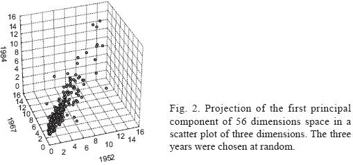
Because there is a significant correlation between years of observation (columns) and considering stations as "observed points", then for any four years, given the precipitation in the three better correlated years, we could estimate the precipitation for the fourth year by means of multiple regression, as an alternative method of choosing the three closest stations in space and estimate missing data from the three stations, a practice accepted in meteorology. Figure 2 shows a scatter plot for three years chosen at random; the points are arranged around a straight line, which represents the projection of the 56 dimensional space of precipitation in a three-dimensional space. Each station represents a point in the graph.

3.2 Cluster analysis

The sample of 349 stations was divided in five clusters, following Englehart and Douglas (2002). The k-means clustering method was then used. This procedure puts the points together in such a way that variability within groups is minimal and variability between groups is maximized (Everitt et al., 2001; Everitt, 2005). This grouping of stations is basically a map of rainfall totals and observed rainfall gradients.

The grouping was made with the daily precipitation averaged during the complete year. As shown in Figure 3 it is possible to differentiate four groups that are spatially coherent and a group of greater precipitation that was not coherent. The groupings show areas of low rainfall in northwestern Mexico, and moderate rainfall in central Mexico, the Gulf of Mexico coastal area, the western state of Nayarit, the Yucatán peninsula and southern Mexico. Rainfall is highest on the slopes of the Sierra Madre Oriental and the extreme values occur at points of Chiapas, Oaxaca, Veracruz and Puebla. This classification shows some features of the climate in the country: dry climates are located in the north, where rainfall is a winter regime, while the southern part of the country is dominated by humid and rainy summers. Additionally, the highest rainfall areas are those in which the rainfall occurs during the entire year (García, 1988).

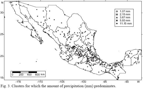
The higher rainfall areas in Mexico are associated with the Sierra Madre Oriental, the Sierra Madre Occidental and Sierra Madre del Sur due to the orographic effect and the contribution of moisture from the oceans surrounding the country. The Northwest is under the influence of subtropical high pressures in the Pacific Ocean, which brings dry air from the north of the continent resulting in an arid climate. In the North the precipitation decreases substantially towards the interior of the country between the Sierra Madre Oriental and the Sierra Madre Occidental due to the Föen effect. In this area the summer rainfall is low and due to the monsoon (Douglas et al., 1993). In summer the southeast is under the influence of the inter-tropical convergence zone and in winter the cold air coming from the north also influences the production of rain during the entire year. Around the Gulf of Mexico, the trade winds are the cause of abundant summer rain. In winter, rains are caused by the orographic effect and the north wind, associated with cold fronts that bring moisture from the Gulf of Mexico. This is expressed in the precipitation maps prepared by García and Mosiño (1990).

Tropical cyclones represent special events, even though isolated, of heavy rain; the most affected states are Quintana Roo, Veracruz and Tamaulipas on the Gulf of Mexico, and Baja California Sur and Sinaloa on the Pacific coast. The months of greatest activity are September and October for both oceans (Azpra et al., 2001).

Comparing the maps prepared by García and Mosiño (1990) there is great similarity between the clusters obtained through the k-means method and the isohyets drawn on a map of annual rainfall mode.

Figure 4 shows the average precipitation arranged from lowest to highest for the 349 stations. This graph represents the empirical probability distribution, which is fitted approximately by a lognormal distribution. If natural logarithms are obtained from the original data, mean and standard deviation are 0.750 and 0.653, respectively. A lognormal distribution simulated with these values is also shown in Figure 4. Chi square and Kolmogorov-Sminov tests showed that it was not possible to reject the hypothesis of a lognormal distribution for the stations.

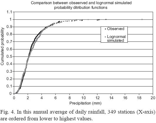
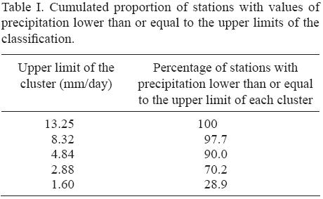
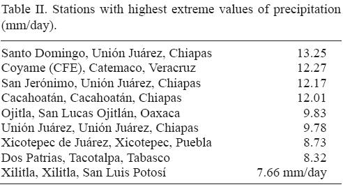
Table I shows the cumulated proportion of stations with precipitation lower than or equal to the upper values of the cluster classification. Stations with the highest values of precipitation are displayed in Table II.

Using the matrix of anomalies of the precipitation with respect to the mean of each station we calculated the covariance matrix and their principal components. The first principal component explains 10.1% of the variance, and the correlation coefficient of the coordinates of the principal component with the variance of the anomalies is –0.7955. Thus, after removing the amount of precipitation, we can identify the first principal component with the variance of each station. After eliminating the amount of precipitation, the result of stations grouping is shown in Figure 5.

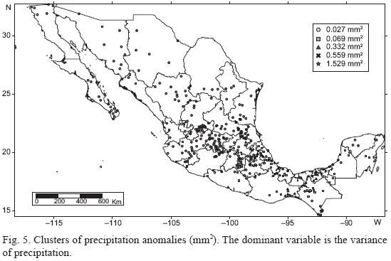
The variance displays a similar pattern to that of the precipitation, which suggests that both are related. The correlation between the variance and the precipitation is 0.779. Southeastern Mexico is the region with larger variance in precipitation.

For the third analysis we eliminate the effect of the variance in clustering by standardizing the precipitation anomalies with the standard deviation of each season. The resulting clustering is shown in Figure 6.

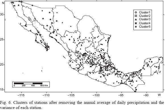
In northern and central regions, a better definition is achieved under this transformation made in terms of rainfall characteristics (trend, response to changes of temperature in the Pacific Ocean, years of maxima and minima). Cluster 1 corresponds mainly to the south, the southeast, and the southern Pacific coast, and some of its stations protrude into areas of clusters 2 and 4. Cluster 2 is clearly located in the center of Mexico, cluster 3 is in the north-central part, cluster 4 corresponds to Sierra Madre Oriental, and finally cluster 5 is located in northwestern Mexico. There are seven stations near the coast of Yucatán Peninsula with grouping characteristics that correspond to the northwest region. This common characteristic is also present in the statistical significance of the relation between ENSO and precipitation (Bravo et al., 2010). This feature could be attributed to the fact that precipitation in the northwest during winter is caused by the arrival of cold fronts to northwestern Mexico and to the Gulf of Mexico (Magaña, 2004).

3.3 Principal component analysis in S mode

For the analysis of the principal components in the S mode, transposing of the matrix of observations is required. In this case we have 349 variables (stations or columns) with 56 cases (years or rows), i.e. a space of 349 dimensions and 56 points. As in the previous case, five principal components were retained. The correlation matrix was used so the precipitation values for each station were centered and standardized. The characteristic values and explained variance are shown in Table III.

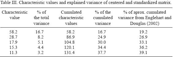
The lower eigenvalues explain less than 3.2% of the variance. The explained variance by the principal components in this work is not very different from that reported by Englehart and Douglas (2002); the difference is probably due to the different sample of selected stations.

Varimax rotation was carried out to obtain the maximum and minimum values for the factor loadings on each axis of factors. The limit value for the factor loadings on each station to be classified in each group was 0.300. Some stations could belong to more than one group and others could not be classified by their low values for factor loadings. The classification is shown in Figure 7. It should be remembered that an increase in station numbers in a high density distribution increases covariance and hence raises the importance of that principal component. The principal components solution could be skewed to the uneven density of stations. Englehart and Douglas (2002) used a more uniform distribution of stations in the Mexican territory. After varimax rotation the grouping skew is reduced. The final grouping is similar to that of Englehart and Douglas despite the skew effect. It is clear that grouping is not dominated by the density of stations. In this case climate dominated the results and the station density had little effect. This can also be seen because some groups have spatial elongated forms with stations separated by long geographical distances.

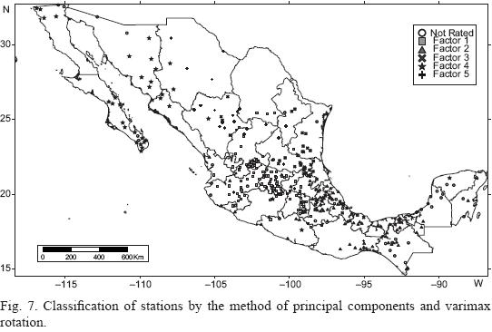
The classification is similar to that made by k-means after standardizing the series (Fig. 6). In Figure 7 the rotated principal component analysis indicates three major regions of precipitation characteristics in northern Mexico: one cluster in the west, which is dry and connected to the descending branch of the Pacific subtropical high (Mosiño and García, 1974; Vázquez et al., 2003; Barry and Chorley, 2010); a second one in the center, between Sierra Madre Occidental and Sierra Madre Oriental; and the third one bordering the Gulf of Mexico, with a higher amount of rainfall associated with the rise of humid air from the sea. The other two conglomerates correspond to central and southern Mexico. The stations that were not classified seem to form a conglomerate in south and southeast Mexico. The comparison of the groupings in this paper with the clustering of Englehart and Douglas (2002) is summarized in Table IV.

The comparison indicates that regions are invariant in time and space and are independent of the method of aggregation and the stations sampled.

3.4 Characteristics of the clusters

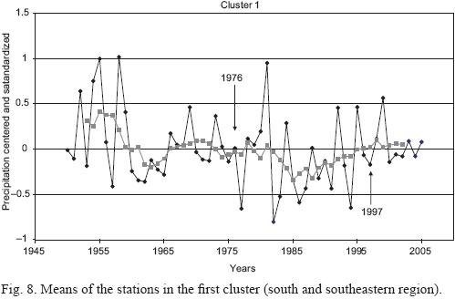
The characteristics of the stations that yield clustering with the use of standardized and cluster analysis data are shown in Figures 8 through 12. (9, 10, 11). Unweighted moving averages using seven values were calculated to smooth the graphs (pink line).

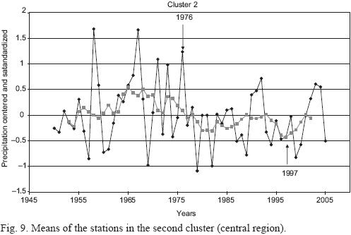
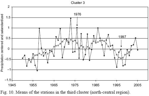
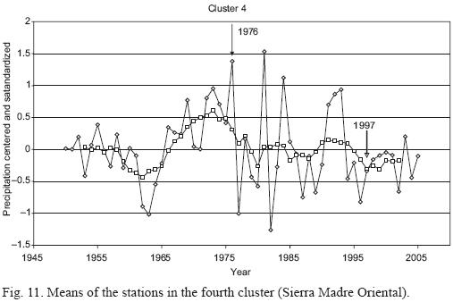
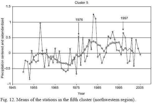
Clusters 2, 4 and 5 show a noticeable change in the behavior of the series during the 1970s. In particular, clusters 2 (central region) and 5 (northwestern region) show a change in structure after 1976, the year in which the change of the cold to the warm phase of the Pacific Decadal Oscillation started (Hare and Francis, 1995). Cluster 2 (central region) shows an abrupt decrease in precipitation level starting in 1976 and cluster 5 (northwestern region) shows an increase in precipitation. Cluster 4 (Sierra Madre Oriental region) shows a change in the variance of the series.

Moving averages show a decrease of the precipitation trend for clusters 2, 3 and 4 during the period 1976 to 1997 (an interval of positive values in the PDO index). From 1950 to 1975 and from 1998 to 2005 (periods of negative PDO values) the trend is an increase in precipitation. However the differences of precipitation between periods of positive and negative values in the PDO index are non-significant. We performed a t-test and a Mann-Whitney U test (Conover, 1971) after grouping stations for negative and positive PDO values, and both gave non-significant results. The behavior of clusters 1 and 5 is different: cluster 1 had a stable mean value without remarkable trends during the study period and cluster 5 had a remarkable and sudden trend for increasing precipitation from 1972 to 1981, as well as a decrease starting in 1995. U-tests and t-tests were non-significant for cluster 1, but the difference was statistically significant for cluster 5 (t-test p <0.0005 and U test p <0.0008). Diagrams of boxes and whiskers are shown in Figure 13.

 

4. Conclusions

We made a careful selection of 349 stations that had 35 to 40 full years of daily rainfall observations. The grouping of stations with principal component analysis highlighted distinct regional behaviors in Mexican precipitation.

The results of the cluster analysis explain satisfactorily the influences of synoptic-scale weather systems and orographic features. The regions in which the Mexican territory was divided by k-clustering and principal component analysis are similar to the results reported by Englehart and Douglas (2002). Two clusters occupy the northwest and north-central part of the territory; there is another defined conglomerate in the center part of Mexico, and the region of the Sierra Madre Oriental forms one more cluster which merges with the southern cluster. In the Yucatán Peninsula some stations behave in a similar way to the northwest cluster, probably due to the occurrence of precipitation in the Northwest during winter caused by the arrival of cold fronts to the area and to the Gulf of Mexico.

There is a strong correlation between years of observation. Therefore, for any four years, given the precipitation in the three better correlated years, we estimate the precipitation for the fourth year by means of multiple regression, using the proximity in precipitation of stations instead of geographical proximity.

In the Mexican territory there were six states with extreme rainfall during the period of observations: Chiapas, Oaxaca, Veracruz, Puebla, Tabasco and San Luis Potosí. It is not possible to reject the hypothesis that the distribution of average precipitation over the period of observations in the sample of stations follows a lognormal distribution.

With raw data, cluster analysis grouping is dominated by the amount of precipitation, which is the variable that dominates the variability of stations. After eliminating the amount of precipitation the grouping is dominated by the variance. By removing the variance, stations are grouped according to features like trend and structural changes of each cluster's series. These characteristics are shown in the graphs of the series. The grouping could be skewed due to the uneven distribution of stations, yet the geographical proximity of stations is not a dominant factor in grouping since there are irregular shaped groups with stations separated geographically. Comparison of the clustering in this work with that of Englehart and Douglas (2002) indicates that the regions and explained variance of each principal component are invariant in time and space, and are independent of the method of aggregation and of the stations sampled. The differences are probably due to the different stations sampled.

As could be expected, the variance is not uniform; it depends on the magnitude of the precipitation. This implies that stations with high or extreme precipitation have also great variability. Stations with low precipitation have also small variations (i.e., the arid zones are consistently arid).

Clusters 2, 3 and 4 show a decreasing trend of precipitation during the period 1976 to 1997 (an interval of positive PDO values). From 1950 to 1975, and from 1998 to 2005 (periods of negative PDO values) there is an increasing trend of precipitation.

The trend is statistically significant only for cluster 5, i.e. northwestern Mexico is the most affected area by the Pacific Decadal Oscillation. With the exception of cluster 5, average precipitation behaved without a definite trend from 1950 to 2005 (von Storch and Zwiers, 1999).

 

Acknowledgements

We thank Ms. in G. Lourdes Godínez for elaborating the figures and Ph. D. Juan Manuel Espíndola for his valuable suggestions and help in correcting the paper.

 

References

Azpra, R. E., A. G. Carrasco, D. D. O. Delgado and C. F. J. Villicaña, 2001. Los ciclones tropicales de México. México: UNAM, Instituto de Geografía, Plaza y Valdés, 120 pp. (M. E. Hernández Cerda, coord. Temas selectos de geografía de México. I. Textos monográficos. 6. Medio ambiente).         [ Links ]

Barry R. G. and R. J. Chorley, 2010. Atmosphere, Weather and Climate. 9th ed. London: Routledge, pp. 163-207.         [ Links ]

Bravo J. L., H. Bravo, P. Sánchez and R. Sosa, 2009. Precipitations trends and floods, in Tabasco, Mexico. Climatic change? Paper 2009-A-632-AWMA. 102nd Annual Conference and Exhibition of the Air & Waste Management Association. Detroit, Michigan.         [ Links ]

Bravo J. L., E. Azpra, V. Zarraluqui, C. Gay and F. Estrada, 2010. Significance tests for the relationship between "El Niño" phenomenon and precipitation in Mexico. Geofis. Int. 49, 245-261.         [ Links ]

Conabio, 2000. Mapas de cabeceras municipales. Comisión Nacional para el Conocimiento y Uso de la Biodiversidad. http://www.conabio.gob.mx/informacion/gis/layouts/cabmun2kgw.gif.         [ Links ]

Conover, W. J., 1971. Practical nonparametric statistics. New York: Wiley.         [ Links ]

Douglas M. W., R. A. Maddox, K. Howard and S. Reyes, 1993. The Mexican monsoon. J. Climate 6, 1665-1667.         [ Links ]

Englehart P. J. and A. V. Douglas, 2002. Mexico's summer rainfall patterns: an analysis of regional modes and changes in their teleconectivity. Atmósfera 15, 147-164.         [ Links ]

Everitt B. S., 2005. An R and S-PLUS companion to multivariate analysis. London: Springer (Springer texts in statistics).         [ Links ]

Everitt B. S, S. Landau and M. Leese, 2001. Cluster Analysis. 4th ed. London: Arnold.         [ Links ]

García E., 1988. Modificaciones al sistema de clasificación climática de Köppen para adaptarlo a las condiciones de la República Mexicana. 4ª ed. México: Offset Larios.         [ Links ]

García, E. and P. Mosiño, 1990. Moda o valores más frecuentes de precipitación mensual y anual. In: A. García de Fuentes, ed. Atlas nacional de México. Vol. II, cap. IV, núm. 4.10. México: UNAM, Instituto de Geografía (escala 1:16 000 000).         [ Links ]

Hare, S. R. and R. C. Francis, 1995. Climate change and salmon production in the northeast Pacific Ocean. Climate change and northern fish populations. Can. Spec. Publ. Fish. Aquatic. Sci. 121, 357-372.         [ Links ]

Jambu, M., 1991. Exploratory and Multivariate Data Analysis. London: Academic Press.         [ Links ]

Jolliffe, I. T., 2002. Principal Component Analysis. New York: Springer Verlag.         [ Links ]

Magaña Rueda, V., ed., 2004. Los impactos de "El Niño" en México. México: UNAM, Centro de Ciencias de la Atmósfera, Secretaría de Gobernación, 229 pp.         [ Links ]

Marcoulides, G. A. and S. L. Hershberger, 1997. Multivariate Statistical Methods: A First Course. Mahwah, NJ: Lawrence Erlbaum Associates.         [ Links ]

Morrison, D. F., 1990. Multivariate Statistical Methods. New York: McGraw-Hill.         [ Links ]

Mosiño A. P. and E. García, 1974. The climates of Mexico. In: R. A. Bryson and F. K. Hare, eds. The Climates of North America. World Survey of Climatology. Amsterdam: Elsevier.         [ Links ]

Türkeş, M. and H. Tatli, 2010. Use of the spectral clustering to determine coherent precipitation regions in Turkey for the period 1929-2007. Int. J. Climatol. 31 (14), 2055-2067. DOI: 10.1002/joc.2212.         [ Links ]

Vázquez M. C., W. Douglas Michael, A. Hahmann, D. Gutzler, J. Shuttleworth, D. Stensrud, J. Amador, R. Carbone, R. Lobato, J. Meitin, C. Ropelewski, J. Schemm, S. Schubert, C. Zhang, R. Wayne Higgins, E. H. Berbery and A. Douglas, 2003. Progress in Pan-American CLIVAR research: The North American monsoon system. Atmósfera 16 (1), 29-63.         [ Links ]

Vidal, R. 2004. Las regiones climáticas de México. México: UNAM, Instituto de Geografía.         [ Links ]

Von Storch, H. and F. W. Zwiers, 1999. Statistical Analysis in Climate Research. New York: Cambridge University Press, p. 114.         [ Links ]

WMO, 2007. Climate Computing Project (CLICOM). World Meteorological Organization. http://www.wmo.int/pages/prog/wcp/wcdmp/clicom/; http://www.wmo.int/pages/themes/climate/climate_data_management_exchange.php.         [ Links ]