Analysis of interdecadal variability of temperature extreme events in Argentina applying EVT

 

B. Tencer and M. Rusticucci

Laboratorio de Extremos Climáticos en Sudamérica, Departamento de Ciencias de la Atmósfera y los Océanos, Facultad de Ciencias Exactas y Naturales, Universidad de Buenos Aires/CONICET, Ciudad Universitaria, Pabellón II, 2º piso (1428), Buenos Aires, Argentina. Corresponding author: M. Rusticucci; e-mail: mati@at.fcen.uba.ar

 

Received August 31, 2011; accepted June 25, 2012

 

RESUMEN

La frecuencia de ocurrencia de los eventos extremos de temperatura ha sufrido variaciones a lo largo del último siglo: se han observado tendencias positivas significativas en las noches cálidas y tendencias negativas en las noches frías en todo el mundo. En Argentina, la probabilidad de ocurrencia de extremos cálidos anuales de la temperatura máxima disminuyó en las últimas décadas, mientras que hubo un incremento en la probabilidad de ocurrencia de extremos cálidos anuales de la temperatura mínima. El objetivo principal de este trabajo es evaluar la variabilidad interdecadal observada en la distribución de los eventos de temperatura que superan un determinado umbral en cinco estaciones meteorológicas de Argentina durante el periodo 1941-2000, mediante la aplicación de la teoría de valores extremos. La disponibilidad de datos diarios permite el ajuste de la distribución generalizada de Pareto (DGP) a las anomalías diarias de temperatura que exceden el percentil 90 o que no alcanzan el percentil 10 con el propósito de estimar los valores de retorno de los eventos extremos. Las series de anomalías diarias de temperatura se dividen en tres subperiodos consecutivos sin superposición de 20 años cada uno. La DGP se ajusta en cada uno de los tres subperiodos en forma independiente y se comparan los valores de retorno estimados en cada subperiodo. Los resultados muestran que hay una disminución en la intensidad de eventos extremos cálidos durante todo el periodo de estudio, junto con un incremento en su frecuencia de ocurrencia durante los últimos 20 años del siglo XX. Los extremos fríos también muestran una disminución en intensidad. Sin embargo, los cambios en su frecuencia de ocurrencia no son tan consistentes entre las diferentes estaciones estudiadas.

 

ABSTRACT

The frequency of occurrence of temperature extreme events has changed throughout the last century: significant positive trends in warm nights and negative trends in cold nights have been observed all over the world. In Argentina, the probability of occurrence of warm annual extremes of maximum temperature has decreased in the last decades, while there has been an increase in warm annual extremes of minimum temperature. The main objective of this paper is to evaluate observed interdecadal changes in the distribution of temperature events that exceed a fixed threshold in five meteorological stations from Argentina over the period 1941-2000, by applying the extreme value theory (EVT). The availability of daily data allows fitting a generalized Pareto distribution (GPD) to daily temperature anomalies over the 90th or below the 10th percentile, in order to estimate return values of extreme events. Daily temperature anomalies are divided into three consecutive and non-overlapping subperiods of 20 years. GPD is fitted to each subperiod independently and a comparison is made between return values estimated in each subperiod. Results show that there is a decrease in the intensity of warm extreme events during the whole period, together with an increase in its frequency of occurrence during the last 20 years of the twentieth century. Cold extremes also show a decrease in their intensity. However, changes in their frequency of occurrence are not so consistent between the different stations analyzed.

Keywords: Temperature extreme events, generalized Pareto distribution, return values, Argentina.

 

1. Introduction

Extreme climate events have changed in several regions of the world. During the last 50 years of the twentieth century there has been a significant decrease in the annual occurrence of cold nights (daily minimum temperature below the 10th percentile) and a significant increase in the annual occurrence of warm nights (daily minimum temperature above the 90th percentile), while decreases in the occurrence of cold days (daily maximum temperature below the 10th percentile) and increases in hot days (daily maximum temperature above the 90th percentile) are generally less marked (Alexander et al., 2006). However, changes in minimum and maximum temperature cannot be represented by a simple shift of the entire distribution to higher values, because cold extremes have warmed more than warm extremes over the last 50 years (Trenberth et al., 2007).

Extreme temperature events happen throughout the year, having different impacts on the ecosystem. Generally, negative linear trends were obtained in the number of cold nights and warm days per summer, while the number of warm nights and cold days has increased in Argentina (Rusticucci and Barrucand, 2004). But temperature extreme events also present interdecadal variability. Barrucand et al. (2008) found decadal variability modes in temperature extreme values in Argentina, associated with larger scale circulation patterns of variability at high latitudes and sea surface temperature variability at surrounding oceans. Rusticucci and Renom (2008) showed that this decadal variability in temperature extremes leads to substantial changes in teleconnections with sea surface temperature in the Equatorial Pacific, before and after the change point of climate trend that occurred between 1976 and 1977 (Trenberth, 1990). From a methodological point of view, the statistics applied to anomalies of extreme minimum and maximum temperatures constitutes a first step in addressing their social and environmental effects. This strategy also permits to evaluate the severity of episodes in terms of very remarkable departures from expected daily values. Additionally, it is an alternative way of analyzing recorded extreme minimum or maximum temperatures. From an applied point of view, this kind of analysis leads to a better knowledge of daily hot and cold episodes, their statistical distributions and return periods (Serra et al., 2009).

In the analysis of extremes, extreme value theory (EVT) is a useful tool to describe the statistical properties of extreme events as well as a useful paradigm to quantify them (Coles, 2001). EVT aims at describing the tail of the distribution of random variables, and stems from a convergence theorem stating that the distributions of extremes follow generic laws, provided that a few elementary hypotheses are verified (Yiou et al., 2008).

A previous study of extreme events in Argentina, performed on an annual basis by fitting a generalized extreme value (GEV) distribution to annual minimum and maximum temperature extremes, reveals that absolute maximum temperatures greater than 32 ºC are expected at least once a year at any station in Argentina, except in the southern part of the country where this value has a return period of 10 years. More extreme events indicate that maximum temperatures greater than 40 ºC may occur once a year or every five years in the central and northern regions, where temperatures reach the highest values of the country. Minimum temperatures below 0 ºC happen every 2 to 10 years in the northeast and at least once a year in the rest of the country (Rusticucci and Tencer, 2008). However, the authors show that return levels suffered changes due to the 1976-1977 climate shift: a decrease in the probability of occurrence of the highest daily maximum temperature (Tx) was found after 1977, while an increase was seen for the highest daily minimum temperature (Tn) at some regions of Argentina; for cold extremes, both Tn and Tx show an increase in return levels, indicating a decrease in the frequency of occurrence of extreme cold events. A generalized Pareto distribution (GPD) has been used for the analysis of extreme values in meteorology and hydrology, as well as to determine damage caused by these events (Katz et al., 2002; Bordi et al., 2007; Re and Barros, 2009; Unkašević and Tošić, 2009; Kioutsioukis et al., 2010). The GPD approach has advantages over the GEV approach because it permits the consideration of more extreme cases per year. Since daily data are available, the GPD approach is now proposed to analyze decadal variability in the frequency and intensity of temperature values that exceed a fixed threshold at five significant meteorological stations from Argentina.

This paper is organized as follows: data and methodology are described in section 2, results are presented in section 3, and finally a brief summary is given in section 4.

 

2. Data and methodology

A generalized Pareto distribution (GPD) was used to model daily minimum and maximum temperature data series, from five meteorological stations in Argentina during the period 1941-2000. Data was provided by the Servicio Meteorológico Nacional (National Weather Service) and quality controlled by Rusticucci and Tencer (2008). This control consisted of an internal consistency analysis that searched the time series for outliers and indisputable erroneous data (such as Tn greater than Tx). The homogeneity of the maximum and minimum annual means has been analyzed by applying two different tests: the Standard Normal Homogeneity Test (SNHT) (Alexandersson, 1986) and the Buishand (1982) test. These tests showed significant shifts at the 1% level in all stations during the 1970s, especially in the minimum temperature. Other studies show significant changes during this decade, not only in surface temperature but also in sea level pressure, sea surface temperature, air temperature at different levels of the troposphere and precipitation (Trenberth, 1990; Seidel et al., 2004; Huang et al., 2005; Rusticucci and Renom, 2008). Buenos Aires also presented a significant shift in minimum temperature in 1967, which is not associated to any changes registered in the metadata available. At Tucumán a significant change was detected in maximum temperature in 1953, but no major changes are registered in metadata that could explain this shift. On the contrary, Santa Rosa has a registered relocation in 1951, even though no significant shifts were seen by the homogeneity tests at this point. No adjustments were made to the series due to the inhomogeneities found since the results shown in this paper are based on the excesses above a certain threshold, and each threshold is calculated on a 20 year period.

The location of stations is shown in Figure 1. The selection of these particular stations is due to the availability of a long record of daily minimum and maximum temperature that allows the analysis of interdecadal variability in different climate regions of the country. In order to have comparable data throughout the year, each series of temperature was transformed into daily standardized anomalies with respect to the period 1961-1990:

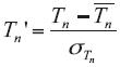
where T_n stands for daily minimum temperature, and are the 1961-1990 minimum temperature mean and standard deviation calculated on a 5-day running window surrounding the day being transformed. An analogous transformation was made for maximum temperature. Therefore, the transformed variables T_n' and T_x' have no units.

With the aim of evaluating interdecadal changes in the period of study, the complete series of anomalies were divided into three non-overlapping consecutive subperiods: 1941-1960, 1961-1980 and 1981-2000. The rationale for choosing 20-yr periods is to retain enough data in each subperiod as to obtain a robust GPD fit but at the same time to be able to characterize interdecadal changes in the extremes. Since stationary data is a requirement of the methodology, significant linear trends at the 95% confidence level were removed from the series of daily standardized anomalies in each 20-yr period using the least square estimation method. A t-Student test showed that this removal does not introduce artificial steps in the time series. The GPD method has two shortcomings that require previous decisions. The first one is the choice of the threshold over which values are considered extreme, since a very low threshold will lead to a violation of the asymptotic hypothesis of the statistical model, while a very high threshold will give weak results due to the few data considered for the analysis. The second one is related to possible non-independent extreme values considered in the analysis, that is, events that are correlated in time.

The first problem was addressed by choosing the 90th (10th) percentile of the distribution of the daily anomalies to be the threshold for the analysis of warm (cold) extremes. This choice was based on the analysis of the goodness-of-fit of the GPD using different thresholds ranging from the 85th to the 99th percentile. Since any of these thresholds led to acceptable fits according to the probability-probability (PP) plots analyzed (not shown), the 90th and 10th percentiles were chosen in order to consider extreme events as those with a probability of occurrence of less than 10%. To solve the second problem, a declustering process is usually applied to data. Here, the declustering process of the daily anomalies was performed by considering only the highest (lowest) value of each five-day period (Jones et al., 1999). That is, whenever two or more excesses were less than five days apart, only the highest (lowest) of all was considered for the analysis of warm (cold) extremes. Therefore, the series of excesses were shortened from 10% of the original data to approximately 5%, defining four variables of extremes: HTn, LTn, HTx and LTx, warm and cold extremes of minimum and maximum temperature, respectively.

A GPD was then fitted to each of the four extreme event series at each station and subperiod using the method of maximum likelihood estimation. Following Coles (2001), the GPD for the random variable y = X – u conditional on X > u, with u being the threshold, is described by the following cumulative distribution function:

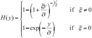
defined only for {y : y > 0 and > 0} with = σ + ξ (u - µ), where µ is the location parameter, σ the scale parameter and ξ the shape parameter. Finally, return levels and their 95% confidence interval were estimated based on the GPD fitted to each subperiod. Following Coles (2001), return levels are defined by

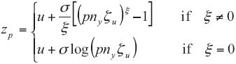
where ζ_u = Pr{X > u} = 0.1 due to threshold choice, n_y is the number of observations per year (365.25 since its daily data) and p is the return period in years. A return value associated with a return period p is a value that is exceeded, on average, once every p years. Return periods can also be expressed as waiting times since the average lapse between two occurrences of a value greater than the corresponding return level is p years. Therefore, changes in return levels indicate changes in the frequency of occurrence of extreme events; and increase in warm/cold extreme return values is associated with an increase/decrease in the frequency of occurrence of warm extremes.

 

3. Results

First of all, interdecadal variability of the complete distribution of extreme events was analyzed. Figure 2 shows the probability distribution function for minimum and maximum temperature anomalies. A shift towards higher Tn values is seen at all stations, especially during the last subperiod. This shift implies an increase both in mean and extreme values. However, changes in mean values are not always consistent with changes at the tail of the distribution. For example, the mean value of maximum temperature at Buenos Aires and Pergamino remained almost constant throughout the period of study while the tails of the distributions are not the same. These differences could be due to changes in the intensity of the extremes or in the frequency of occurrence.

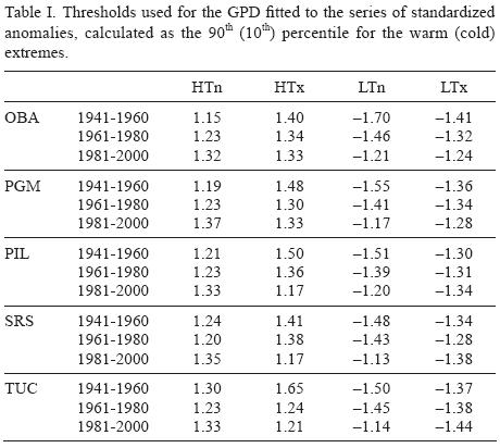
With the aim of studying the observed interdecadal variability in the intensity of extreme temperature events, 10th and 90th percentiles of the empirical distribution were calculated for series of minimum and maximum daily anomalies in each subperiod. These values were then used as thresholds for GPD fit. Figure 3 and Table I show percentiles for the different stations, subperiods and variables. Warm extreme events in maximum temperature (Fig. 3b) and cold extremes in minimum temperature (Fig. 3c) are the events that show greater changes, with a decrease in the first case, and an increase in the latter, most noticeable in the last subperiod. Since the 10th (90th) percentile indicates the magnitude of the lower (upper) 10% tail of the distribution, an increase (decrease) in this value implies a decrease in the intensity of cold (warm) extremes. Changes in warm extremes of minimum temperature and cold extremes in maximum temperature (Figs. 3a and 3d, respectively) do not show important changes throughout the period, although a general increase in the 90th percentile is seen in minimum temperature at all stations, especially during the last subperiod, indicating an increase in the intensity of warm events. Changes in the 10th percentile of maximum temperature depend on the station. The maximum absolute difference between the first and last subperiod is 0.5 standard deviations from the mean in maximum temperature warm extremes and minimum temperature cold extremes, and less than 0.2 standard deviations in the other events. The large difference seen in Tucumán between the first and the following subperiods could be due to the lack of homogeneity detected in 1953. However, since the following analyses will be applied to excesses above this threshold, this lack of homogeneity should not introduce uncertainties on the results.

A GPD was then fitted to the series of minimum and maximum temperature anomalies at each station and subperiod using the 10th (90th) percentiles as the threshold for cold (warm) extremes. Parameters were estimated by the maximum likelihood method, and goodness-of-fit was analyzed by PP plots (not shown). Changes in return values for each subperiod were then calculated in order to analyze interdecadal variability in the frequency of occurrence of daily extreme events.

Figure 4 shows 20-yr return values of standardized anomalies of minimum and maximum temperature extreme values for each station and subperiod. Warm extremes (Figs. 4a and 4b) show a decrease in the 20-yr return value from the first (1941-1960) to the second (1961-1980) subperiod, that is, a decrease in the frequency of occurrence of warm extremes. However, during the last subperiod (1981-2000) an increase in this value followed at all stations, except at Santa Rosa (HTx). This increase, that in most cases resulted of greater magnitude than the decrease observed before, leads to an increase in the frequency of occurrence of warm extremes during the last 20 years of the twentieth century, both in minimum and maximum temperature. Changes are of the order of 0.5 standard deviations from the mean, and up to one standard deviation, however not significant at the 5% level due to superimposition of 95% confidence intervals in almost all the cases. Cold extremes show smaller (not significant) changes, not consistent along all the stations. The magnitude of these changes varies from 0.2 to 0.7 standard deviations from the daily mean. In particular, return values of minimum temperature cold extremes (Fig. 4c) increased at Pergamino, Pilar and Santa Rosa, while at Buenos Aires an increase in the second subperiod was followed by a greater increase in the last subperiod, and the opposite occurred at Tucumán.

These changes in return values can also be expressed as waiting times or return periods. Table II shows the 20-yr return value of the standardized daily anomalies drawn from the GPD fitted to the first subperiod (1941-1960) at each station (first row). Waiting times for that specific value were then calculated from the GPD fitted to the following subperiods (second and third rows). Consistently with Figure 4, waiting times are greater than 20 years where return levels of warm extremes have decreased, and lower than 20 years where return levels have increased. The opposite occurs for cold extremes.

 

4. Summary and conclusions

Four variables were defined here to describe extreme temperature events: HTx, HTn, LTx and LTn represent independent anomalies of the lowest and highest minimum and maximum temperature and are based on the series of daily data. A GPD has been fit to each variable in different subperiods to analyze interdecadal variability in the frequency and intensity of temperature extreme events in some significant regions of Argentina. This statistical analysis shows that extreme events have changed both in intensity and frequency of occurrence, not only due to a linear trend as was shown by Rusticucci and Barrucand (2004), but also on decadal timescales. The intensity of maximum temperature warm extreme events (HTx) and minimum temperature cold extreme events (LTn) decreases over the period 1941-2000, while minimum temperature warm extreme (HTn) intensity has increased at all stations, though this change is of less magnitude.

Regarding the frequency of occurrence of extremes, warm extreme events (both for minimum and maximum temperature) showed a decrease from 1941-1960 to 1961-1980, followed by an increase in the last 20 years of the twentieth century, except for HTx at Santa Rosa where this increase is not seen. This implies an increase in the frequency of occurrence of warm temperature extreme events during the last period. The station with the greatest changes is Pergamino, with increases of almost one standard deviation from the daily mean. However, these changes are not significant due to superimposition of the 95% confidence intervals in almost all cases. Cold extreme events of maximum temperature did not change consistently at the different stations studied, and presented smaller changes than warm extremes.

Overall, the frequency of occurrence of warm extremes decreased (lower waiting times) during 1961-1980 with respect to the previous subperiod, but increased again in the last 20 years of the twentieth century, even to higher frequencies than the observed before. Cold extremes showed mostly a decrease in their frequency of occurrence in the last subperiod at almost all stations.

 

Acknowledgments

This work has been partly funded by the following projects: UBACYT X170, CONICET PIP 0227 and the CLARIS LPB Project of the Seventh Framework Programme (a Europe-South America network for climate change assessment and impact studies in La Plata Basin).

 

References

Alexander L. V., X. Zhang, T. C. Peterson, J. Caesar, B. Gleason, A. M. G. Klein-Tank, M. Haylock, D. Collins, B. Trewin, F. Rahimzadeh, A. Tagipour, K. Rupa-Kumar, J. Revadekar, G. Griffiths, L. Vincent, D. B. Stephenson, J. Burn, E. Aguilar, M. Brunet, M. Taylor, M. New, P. Zhai, M. Rusticucci and J. L. Vázquez-Aguirre, 2006. Global observed changes in daily climate extremes of temperature and precipitation. J. Geoph. Res. 111, D05109. DOI:10.1029/2005JD006290.         [ Links ]

Alexandersson H., 1986. A homogeneity test applied to precipitation data. J. Climatol. 6, 661-675.         [ Links ]

Barrucand M., M. Rusticucci and W. Vargas, 2008. Temperature extremes in the south of South America in relation to Atlantic Ocean surface temperature and Southern Hemisphere circulation. J. Geoph. Res. 113, D20111. DOI:10.1029/2007JD009026.         [ Links ]

Bordi I., K. Fraedrich, M. Petitta and A. Sutera, 2007. Extreme value analysis of wet and dry periods in Sicily. Theor. Appl. Climatol. 87, 61-71.         [ Links ]

Buishand T. A., 1982. Some methods for testing the homogeneity of rainfall records. J. Hydrol. 58, 11-27.         [ Links ]

Coles S., 2001. An introduction to statistical modeling of extreme values. Great Britain: Springer, 208 pp.         [ Links ]

Huang H. P., R. Seager and Y. Kushnir, 2005. The 1976/77 transition in precipitation over the Americas and the influence of tropical sea surface temperature. Clim. Dynam. 24, 721-740.         [ Links ]

Jones P. D., E. B. Horton, C. K. Folland, M. Hulme, D. E. Parker and T. A. Basnett, 1999. The use of indices to identify changes in climatic extremes. Climatic Change 42, 131-149.         [ Links ]

Katz R. W., M. B. Parlange and P. Naveau, 2002. Statistics of extremes in hydrology. Adv. Water Resour. 25, 1287-1304.         [ Links ]

Kioutsioukis I., D. Melas and C. Zerefos, 2010. Statistical assessment of changes in climate extremes over Greece (1955-2002). Int. J. Climatol. 30, 1723-1737.         [ Links ]

Re M. and V. R. Barros, 2009. Extreme rainfalls in SE South America. Climatic Change 96, 119-136.         [ Links ]

Rusticucci M. and M. Barrucand, 2004. Observed trends and changes in temperature extremes over Argentina. J. Climate 17, 4099-4107.         [ Links ]

Rusticucci M. and B. Tencer, 2008. Observed changes in return values of annual temperature extremes over Argentina. J. Climate 21, 5455-5467. DOI: 10.1175/2008JCLI2190.1.         [ Links ]

Rusticucci M. and M. Renom, 2008. Variability and trends in indices of quality controlled daily temperature extremes in Uruguay. Int. J. Climatol. 28, 1083-1095. DOI:10.1002/joc.1607.         [ Links ]

Seidel D. J., J. K. Angell, J. Christy, M. Free, S. A. Klein, J. R. Lanzante, C. Mears, D. Parker, M. Schabel, R. Spencer, A. Sterin, P. Thorne and F. Wentz, 2004. Uncertainty in signals of large scale climate variations in radiosonde and satellite upper-air temperature datasets. J. Climate 17, 2225-2240.         [ Links ]

Serra C., M. D. Martínez, X. Lana and A. Burgueño, 2009. Extreme normalized residuals of daily temperatures in Catalonia (NE Spain): sampling strategies, return periods and clustering process. Theor. Appl. Climatol. 101, 1-17. DOI:10.1007/s00704-009-0172-3.         [ Links ]

Trenberth K. E., 1990. Recent observed interdecadal climate changes in the Northern Hemisphere. B. Am. Meteor. Soc. 71, 988-993.         [ Links ]

Trenberth K. E., P. D. Jones, P. Ambenje, R. Bojariu, D. Easterling, A. Klein Tank, D. Parker, F. Rahimzadeh, J.A. Renwick, M. Rusticucci, B. Soden and P. Zhai, 2007. Observations: Surface and atmospheric climate change. In: S. Solomon, D. Qin, M. Manning, Z. Chen, M. Marquis, K. B. Averyt, M. Tignor and H. L. Miller, eds. Climate Change 2007: The Physical Science Basis. Contribution of Working Group I to the Fourth Assessment Report of the Intergovernmental Panel on Climate Change. Cambridge: Cambridge University Press, 11 pp.         [ Links ]

Unkasevic M. and I. Tosic, 2009. Changes in extreme daily winter and summer temperatures in Belgrade. Theor. Appl. Climatol. 95, 27-38. DOI:10.1007/s00704-007-0364-7.         [ Links ]

Yiou P., K. Goubanova, Z. X. Li and M. Nogaj, 2008. Weather regime dependence of extreme value statistics for summer temperature and precipitation. Nonlinear Processes Geophys. 15, 365-378.         [ Links ]