Implementation and applications of chaotic oscillatory based neural network for wind prediction problems

 

K. M. KWONG, F. W. TEE, J. N. K. LIU
Department of Computing, the Hong Kong Polytechnic University, 11 Yuk Choi Road, Hung Hom, Kowloon, Hong Kong, China Corresponding author K.M. Kwong; e–mail: kaming.kwong@gmail.com

 

P. W. CHAN
Hong Kong Observatory, 134A Nathan Road, Kowloon, Hong Kong, China

 

Received September 22, 2010; accepted April 1, 2011

 

RESUMEN

La cizalladura del viento y los cambios repentinos en su direccióny velocidad son un peligro familiar para la aviación, así como un fenómeno complejo y difícil de predecir. Las causas de las cizalladuras pueden variar según el lugar. En algunos sitios se deben a reventones, columnas localizadas de aire descendente, mientras que en otros lugares las cizalladuras pueden ser consecuencia de fenómenos meteorológicos de mesoescala. Por lo tanto, los algoritmos y técnicas que se utilizan para predecir las cizalladuras del viento causadas por reventones, como en Wolfson et al. (1994), no serán aplicables en un aeropuerto donde la cizalladura del viento y la turbulencia surgen de las condiciones locales pero de escala mayor. Este trabajo presenta la implementación y aplicación de redes neuronales caóticas oscilatorias (CONN) para predecir la brisa marina y la cizalladura del viento que se originan en los fenómenos meteorológicos de mesoescala en el Aeropuerto Internacional de Hong Kong. Utilizando datos históricos locales proporcionados por el Observatorio de Hong Kong se muestra, a partir de simulaciones, que CONN es capaz de predecir los movimientos del viento y hasta cizalladuras con un nivel razonable de precisión.

 

ABSTRACT

Wind shear, sudden change in the wind direction and speed, is a familiar hazard to aviation as well as a complex and hard-to-predict phenomenon. The causes of wind shear may be different in different locations. In some places it is caused by microbursts, viz. localized columns of sinking air brought by thunderstorms, while in other places wind shear may result from mesoscale weather phenomena. Thus, algorithms and techniques used to predict wind shear caused by microbursts, as in Wolfson et al. (1994), will not be applicable at an airport where wind shear and turbulence arise from larger-scale but local conditions. This paper presents the implementation and applications of chaotic oscillatory-based neural networks (CONN) forpredicting seabreeze and wind shear arising from mesoscale weather phenomenon at the Hong Kong International Airport. Using historical local data provided by the Hong Kong Observatory, we show from simulations that CONN is able to forecast the short-term wind evolution and even wind shear events with a reasonable level of accuracy.

Keywords: Chaotic oscillator, neural network, wind shear, forecast.

 

1. Introduction

The term wind shear refers to a change in the wind direction and speed that typically lasts from 3 to 40 seconds and results in a sustained change in the headwinds experienced by aircraft. A decrease in headwind will result in decreased lift and this in turn may mean that an aircraft fails to fly at its planned flight path (HKO, 2010).

While wind shear is a familiar hazard to aviation, it is also a complex and hard-to-predict phenomenon. One particular difficulty is that the causes of wind shear may be different in different locations. In some places wind shear is caused by microbursts, viz. localized columns of sinking air, while in other places wind shear may result from mesoscale weather phenomena associated with seasonal prevailing winds and local topographies. Thus, algorithms and techniques used to predict wind shear caused by microbursts, as in Wolfson et al. (1994), will not be applicable at an airport such as Hong Kong International Airport (HKIA), where the main causes of wind shear and turbulence are strong winds blowing across the local hills (Pérez-Munuzuri et al., 1996; Shun, 2004), the disturbed airflow associated with tropical cyclones, and the fact that at HKIA winds turn westerly over the western part of the coastally-sited airport in an environment of prevailing easterly winds due to sea breeze (HKO, 2010). Wind shear is not uncommon at HKIA, where it is experienced at significant level by about one in 500 arriving and departing flights and as moderate to severe turbulence in around one in 2000 flights, with many occurrences being in non-rainy and clear-air conditions (HKO, 2010).

A further difficulty in the prediction of wind shear is that it is hard to model, not least because it arises over very short time periods. Artificial Neural Networks (ANN) have been applied with success to various time series prediction problem and even weather prediction problems, and may be useful in this regard.

Han et al. (2004) try to model and predict chaotic series based on a recurrent predictor neural network. Wang and Fu (2005), and Wang et al. (2001) present the use of fuzzy neural networks, multi-layer perceptor neural networks (MLP) and radial basis function neural networks in data dimensionality reduction, classification, and rule extraction. Castillo and Melin (2002) make use of hybrid intelligent systems for the estimation of the fractal dimension of a geometrical object. On the other hand, Mitra et al. (2010) used neural network approach for temperature retrieval. Bilgili et al. (2007) used hourly mean wind speeds and ANN to predict mean monthly wind speeds. More and Deo (2003) used ANN and wind forecasts to predict the power output of wind turbines. Öztopal (2006) used ANN in predicting the wind potential of various regions. Barbounis et al. (2006) used ANN to forecast long-term wind speeds and their potential for use in generating wind power. In all of these cases, however, the predictions were only of mean hourly or monthly wind velocities and covered relatively large regions, making them inapplicable to very short time frames and localized considerations of airport wind shear problems.

One way to deal with the short-term nature of wind shear prediction is to apply chaotic neural networks (Kwong et al., 2008; Wong etal., 2008) which model the non-linear behavior of neurons, activating a neuron with a non-linear output function, thereby providing for much more complex behavior than the simple thresholds functions used in conventional ANN. Chaotic behavior offers weather forecasting with a rich library of useful behaviors (Zhang et al., 1998). Neural network architectures and learning algorithms involving chaos have been used for the storage in memory of analog patterns (Imai etal., 2005). While it is hard to apply chaos theory to long-term prediction, it seems that, owing to its ability to focus on the simple deterministic relationships between what would appear to be random-looking data, it may be well-suited to short-term prediction, especially when a good model is lacking (Zeng et al., 1993).

In this paper, we propose two applications that use chaotic oscillatory-based neural networks (CONN) to forecast the evolution of winds along the glide path and runway. One proposed application makes use of wind data measured by an automatic weather station (AWS) for the sea breeze forecast, while another makes use of accurate Doppler velocities measured by using LIDAR (Light Detection And Ranging data). Those data were collected by Hong Kong Observatory (HKO) at HKIA.

An AWS enables measurements at remote areas and typically consists of data logger, battery, telemetry and meteorological sensors with an attached solar panel or wind turbine and mounted upon a mast. AWS can measure the meteorological data including temperature, wind speed, wind direction, humidity, pressure, rainfall and visibility.

LIDAR is an optical analogue of RADAR (RAdio Detection And Ranging). It uses a ground-based pulsed laser to measure the velocity of aerosols in the air. LIDAR has previously been used to detect occurrences of wind shear, with high accuracy (Shun and Chan, 2008), but there has been little research into using it to forecast wind shear.

The two proposed applications were tested in simulations and their predictions were compared with historical data. The applications were able to forecast the time, location and magnitude of sea breeze or wind shear event with considerable accuracy. This paper is organized as follows. Section 2b describes chaotic oscillators, which form the basis of our chaotic oscillatory-based neural networks (CONN) approach. Section 2c presents our methodology for applying CONN on wind shear forecasting. Section 3 presents our simulation and simulation results. Section 4 presents our conclusion and an outline for future work.

 

2. Methodology

The paper would discuss a Sea Breeze Forecast System (SBFS) for the forecasting of wind changes associated with sea breeze at HKIA, and a Wind Shear Forecast and Alerting System (WSFAS) for the short-term forecasting of significant windshear due to sea breeze or terrain disruption of the airflow at the airport. Both systems share a similar system architecture, they both contain, i) a series of data preparation processes for data cleaning, filtering, normalization, etc. and ii) Chaotic Oscillatory Based Neural Network as the learning unit and forecast engine. For the WSFAS, there will be a wind shear detection process after the CONN learning and forecast engine for capturing the wind shear events in the forecast.

 

a) Data preparation

We have made use of the data for the wind shear forecast and alerting, including, air temperature, sea temperature, wind direction and wind speed from AWS that is located along the runway for the sea breeze forecast and Doppler velocity data derived from glide path scans of LIDAR for wind shear forecast. These collected meteorological data are processed by different preparation processes before being fed into the CONN model for learning.

The AWS data are pre-processed with those invalid and missing data removed. They are then converted from 1-minute data into 10-minute mean values.

The LIDAR data are pre-processed with quality control algorithm (Chan et al., 2006). Outliers are detected by comparing each piece of radial velocity with neighboring data points. If the difference between them is larger than a predefined threshold, it will be smoothed using a median-filtered value. The threshold is determined from the frequency distribution of the difference in the velocities of the adjacent range/azimuthal gates of the LIDAR over a long period of time. Data quality control is kept to a minimum in order to avoid smoothing out the genuine wind fluctuations of the atmosphere (Chan et al., 2006). If data is missing from a particular location, any available valid velocity data from neighboring positions or time frames is used to derive a replacement velocity value through a linear interpolation of the velocities at the neighboring points.

For the Sea Breeze Forecast System, each set of training data is combined based on the measurement of different AWS located along the runways and sea breeze around the HKIA at the past one hour. The training data including the air temperature, sea temperature, wind direction and wind speed are used to train the model which is expected to capture the see breeze movement, therefore be able to provide prediction for wind direction and wind speed along the runways. The time interval between two training sets is set at 10 minutes; for the WSFAS, each set of training data is for the glide path at a specific time. It includes the Doppler velocities on a slant range, angle of elevation, and azimuth. These are used to train the model to predict Doppler velocities along the glide path in the upcoming three minutes. The time difference between two training sets varies from 3 to 4 minutes.

For both SBFS and WSFAS, the training and testing data sets are normalized between minimum (-1) and maximum (+1) before training and testing of the CONN.

 

b) Chaotic oscillatory based neural network

The CONN is made up of a MLP neural network and a Lee oscillator (retrograde signaling) model (LOM) with various parameter settings. The MLP neural networks are constructed by one or two hidden layers with several neurons, and the activation function of the neurons in the hidden layer(s) and output layer are replaced with the LOM (Fig. 1) rather than with the sigmoid or hyper tangent function as in conventional neural networks.

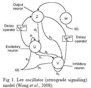
The LOM exhibits chaotic progressive growth in its neural dynamics, it can be used as an effective chaotic bifurcation transfer unit in neural networks. The LOM model consists of the neural dynamics of four constitutive neural elements: u, v, w and z. The neural dynamics of each of these constituent neurons are given by:

where u(t), v(t), w(t) and z(t) are the state variables of, respectively, the excitatory, inhibitory, input and output neurons; f() is the hyperbolic tangent function; a1, a₂, a₃, a₄, b1, b₂, b₃ and b₄, are the weight parameters for these constitutive neurons; θ_u and θ_V are the thresholds for excitatory and inhibitory neurons; I(t) is the external input stimulus, and k is the decay constant.

 

c) Training and testing of the CONN

The CONN is trained with a month of the preprocessed data, which is formatted into time intervals using a back propagation learning algorithm. A momentum term is used to speed up convergence and avoid local minima. It learns from the root mean square error between the predicted result and the measured value from AWS in Sea Breeze Forecast System or LIDAR in WSFAS through back propagation. In the testing process, the neural network uses the experience gained in the training process to generate the forecast for the next time intervals.

Figure 2 shows the structure of the CONN learning unit and forecast engine that have been used in the following simulations. For the SBFS, the meteorological data collected from the AWS located along the runway and the sea around the HKIA in the past one hour are the inputs (Vi_n) to the neurons of input layer. The outputs (V_out) would be the forecast of wind speed and direction in the next time frame at the location of AWS along the runway and around the HKIA. For the WSFAS, the current wind pattern along the selected glide path (Vi_n), which is measured by the LIDAR system, is fed into the CONN through the input nodes in the input layer. The forecast of the winds along the selected glide path (V_out) in the next time frame can be obtained at the output node in the output layer.

For both CONN forecast systems, neurons in hidden layers and output layer produce the output of the chaotic oscillator based on the corresponding external stimulus received from the connected neurons in the previous layer. There can be one to two hidden layers with several hidden neurons within. The number of hidden layers and hidden neurons are chosen experimentally since there is no simple clear-cut method for determining these parameters.

Experiments show that different parameter settings used with the LOM result in different performance in various weather phenomenon. There is only one parameter setting for the Sea Breeze Forecast System; but two different parameter settings are used for the WSFAS. Those parameters used in the SBFS and WSFAS were also chosen experimentally. Table I presents the values of the parameters that are used with the LOM in the hidden layers and output layer of the Sea Breeze Forecast System; while Table II presents the values of the parameter settings that are used with the LOM in the hidden layers and output layer of the WSFAS, which are labeled as characters A and B in the hidden layers and output layer, respectively, in Figure 2.

 

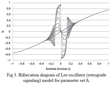
Figures 3 and 4 show the bifurcation diagrams of the LOM with parameter sets A and B. The x-axis represents the external stimulus (I) from the connected neurons in the previous layer to the chaotic oscillator. The y-axis represents the output of the chaotic oscillator corresponding to the external stimulus. The response of the LOM to an external input stimulus with parameter sets A and B can be categorized into two regions, the sigmoid-shape region and the hysteresis region. The former denotes the non-chaotic neural activities in the oscillator. The latter denotes the chaotic behavior that results when a weak external input stimulus is received.

In our previous work (Kwong et al., 2008), the parameters which were used in individual neurons were predefined before the start of training process and the training process only focused on tuning the weights among different layers of neurons. As the shape of the bifurcation is predefined, the responses of the LOM are limited to the outermost shell of the chaotic region.

Neural oscillators depend on parameters that have to be tuned to achieve the desired performance. However, since neural oscillators have highly nonlinear dynamics, parameters of neural oscillators are difficult to tune (Arsenio, 2000, 2004). Although there has been work on chaos control and tuning of the parameters of neural oscillator, most of it concentrates on oscillation control or the frequency, amplitude and phase of the neural oscillator (Arsenio, 2000; Arsenio, 2004; Miyakoshi etal., 2000; Hirasawa etal., 2000). Little work has considered the shape of the bifurcation diagram used as the transfer function in CONN.

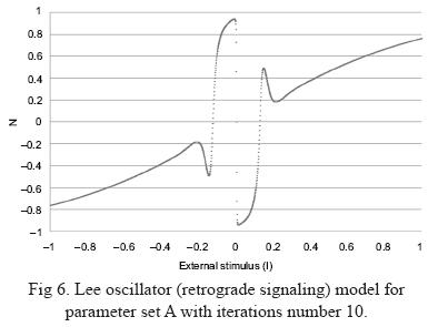
Experimental variation in the number of iterations of the same parameters set during the training process allows CONN to produce different possible changes in the chaotic region of the LOM. Figures 5 and 6 show the appearance of the LOM for parameter set A at iterations 4 and 10.

In order to increase the learning ability and flexibility of the CONN model, the training process of the Wind Shear Forecast and Alerting System not only tunes the bias of neurons and the weights between input layer, hidden layer and output layer, it also adjusts the number of iterations of the LOM in the output layer neurons. As the time required computing the LOM is directly proportional to the number of iterations that are assigned, it is also possible to improve the performance of the CONN, reducing the time required for less necessary iterations by adjusting the number of iterations used in each individual neuron during the training process.

The mechanism is that a randomly generated iterations number (N) will be assigned to each neuron in both hidden and output layers during initialization of the neural network. Neurons in the output layer will produce five different outputs by using the assigned iteration number. For example, if value 10 is assigned to the first neuron in the hidden layer during initialization, this neuron will produce five outputs by using N ± 2 (in this example N = 8, = 9, = 10, = 11 and = 12 are to be used) with the same parameter set in the current epoch of training. After comparing the outputs with the actual measured data from LIDAR, the output with the smallest error value will be selected as the output of that neuron. On the other hand, the N that produces the output with the smallest error will be used to update the old N of that neuron in that training epoch and will be the initial iteration number for that neuron in the next epoch. Once the changes of the iteration number in an individual neuron become steady, the mechanism that updates the iteration number in that neuron will stop. We assume that the neural oscillator used in that neuron is already well trained.

By varying the iteration number, different possible changes in the chaotic region of the chaotic oscillator are tested and selected heuristically in the training process. The use of the chaotic oscillator is no longer limited to the outermost shell of the chaotic region produced by a fixed number of iterations assigned at the initialization of CONN.

 

d) Wind shear detection in the forecast result

The Hong Kong Observatory has developed an algorithm called the GLide-path scan Wind shear alerts Generation Algorithm (GLYGA), which detects wind shear automatically from headwind profiles generated from LIDAR data (Chan et al., 2006; Shun and Chan, 2008). By combining GLYGA and the forecasted results that are produced by CONN, it is possible to forecast wind shear events. We do this by first combining the forecast radial velocities along a glide path to construct a headwind profile. Differences between the velocities of adjacent data points in the headwind profile are calculated to construct a velocity increment profile which is used to magnify the change of velocities and make it easy to capture wind shear ramps, namely, the peaks and troughs in the velocity increment profile. Next, the ramps are detected by comparing each data point of the profile with the neighboring points on two sides. The wind shear ramps detected from a headwind profile are prioritized using a normalized wind shear value AV/H^1/3, suggested by Jones and Haynes (1984), where AV is the total change in the headwind and H is the ramp length. If any one of the wind shear ramps exceeds 14 knots (Shun and Chan, 2008), an alert message is generated.

 

3. Simulation

In this section, we will go through two simulations, one simulation is the forecast of sea breeze by CONN and the other simulation is the forecast of wind shear event by CONN. Reader may refer to our previous work (Kwong et al., 2008) for the comparison of CONN and simple MLP neural network in the wind forecast application.

 

a) Sea breeze forescast by CONN with AWS data

We tested the seabreeze forecast ability of CONN by using atypical seabreeze case on 13 November 2007. As all the AWS worked normally and most of the necessary data were valid for training and testing, it was a good case for catching the sea breeze by using CONN. In order to obtain the optimal learning effort, the data of the whole past month were used as the training data set, and the testing data set was extracted from the AWS database. A set of 4140 training records from 16 October 2007, 05:01:00 (UTC) to 12 November 2007, 16:00:00 (UTC) were used and these data included the air temperature, sea temperature, wind direction and wind speed recorded by the chosen AWS.

The wind barbs in Figure 7 show the wind recorded between the time 13 November 2007,05:50:00 and 06:00:00 (UTC) by the AWS and the numbers beside them are the corresponding temperatures at sea or air. As shown in the wind maps, the overall wind direction is changing from easterly to westerly over the western part of the two runways. Letters A to G in Figure 7 indicate the corresponding location of AWSs that are affected by the sea breeze in the following hour.

In Figure 7a, the wind barb at location A is northward-pointing while the wind barbs at locations B, C, D, E and F are westward-pointing at 04:50:00 (UTC). As the sea breeze starts to affect the glide path at 05:00:00 (UTC) (see part b), the wind barbs at locations A and C change and point toward the northeast; 10 minutes later, the wind barb at location B (see Fig. 7c) changes and points to the northeast. Later on, the sea breeze affects the runway end and changes the pointing direction of wind bards at locations D and E at 05:20:00 (UTC), 05:30:00 (UTC) and 05:40:00 (UTC) as shown in Figures 7d, 7e and 7f, respectively. Finally, the sea breeze passes through the HKIA and changes the pointing direction of wind bards at locations F and G from pointing west to pointing east at 05:50:00 (UTC) and 06:00:00 (UTC), respectively (see Fig. 7g and 7h).

As the change of wind direction is one of the most significant features of sea breeze, the following simulations will focus on capturing the changes of wind direction. The forecast start-time of the testing case was 13 November 2007, 05:00:00 UTC in order to see if the CONN could predict the change of wind direction.

Figures 8 to 10 show the preliminary forecast result from the CONN Sea Breeze Forecast System at three different locations, the western end of the south runway (R1W), the middle of the south runway (R1C) and the eastern end of the south runway (R1E). In Figures 8, 9 and 10, the x-axis presents the time steps in seconds and y-axis presents the wind direction in degrees. Time step 1 means the first time step after the starting time of forecast, i.e. 05:10:00 UTC in the experiment, and each time step is set at 10 minutes after the previous one. The blue lines in the figures show the actual measurement of 10-min averaged wind direction by AWS at different locations (Fig. 8 for location R1W, Fig. 9 for location R1C and Fig. 10 for location R1E). And the red lines show the forecast made by CONN.

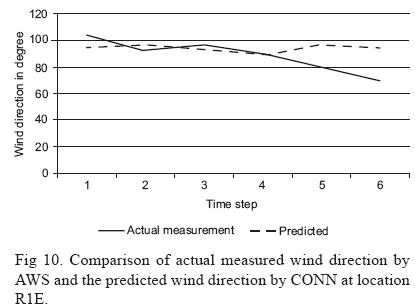
In this simulation, the forecast results produced by CONN are comparable with the actual reading recorded from AWS. The CONN forecasts not only capture the change in wind direction from 100 to 250 degrees between the time steps 2 to 5 as shown in Figures 8 and 9 successfully, but also the steady wind direction in Figure 10. Future studies of short-term forecasting of seabreeze would look at the possibility of forecasting the wind direction change in the airport area before this change takes place over the AWS (weather buoys) to the west of HKIA, as well as retreat of sea breeze over the airport.

 

b) Wind shear forecast by CONN with LIDAR data

We also tested CONN for the wind shear forecast and alert ability by using another set of sea breeze data measured by LIDAR from 6 January 2009. This date was chosen because it was a day of significant wind shear with large wind shear ramps. A training set was constructed from the data recorded by LIDAR between 1 December 2008, 02:42:46 (UTC) and 1 January 2009, 06:03:57 (UTC) and a testing set was constructed from the data recorded between 6 January 2009, 04:03:09 (UTC) and 04:54:58 (UTC).

Figure 11 shows the overall changes of the headwind along the glide path 07RA between 6 January 2009 04:05 (UTC) and 04:53 (UTC). Figure 12 shows the forecast of the headwind profile along the glide path 07RA made using the current CONN model. The x-axis shows the distance from the end of the runway in nautical miles (NM) and the y-axis shows the headwind velocity in meters per second. The various gray lines indicate the wind field along the glide path at different moments.

Figure 13 shows headwind profiles obtained by applying the GLYGA algorithm with the actual observed LIDAR data and simulation results for the seabreeze for the period from 6 January 2009 at the arriving runway corridor 07RA with different time slots. Those small figures on the left are the forecasts made by CONN. The small figures on the right are the actual observations from LIDAR. The x-axis is the distance away from the end of the runway in nautical miles. The y-axis on the left is for the headwind measured in knots. The y-axis on right hand side is the altitude of the glide path measured in feet. The detected wind shear ramp(s) are highlighted.

In this simulation, the forecast predicted most of the actual observed wind shear. In the period between 04:05 (UTC) and 04:56 (UTC) wind shear was successfully forecast for seven out of eight occurrences in 14 time slots. For example, one 14-knot wind shear ramp was observed between 0.3 and 1.4 NM from the end of the runway at 04:17:06 (UTC). The GLYGA algorithm gave a 15-knot wind shear ramp between 0.5 and 1.5 NM from the end of the runway at 04:17:06 (UTC). We also note that the region highlighted in our figures as a predicted wind shear ramp corresponds to the region where wind shear in fact occurred in the observed headwind profiles and were of a similar magnitude. In short, the CONN model was able to make good predictions of the incidence of both particular wind shear events and of the general location and magnitude of occurrences. Figure 14 provides a scatter diagram comparing the observations and forecasts between 6 January 2009 04:05 (UTC) and 04:56 (UTC). The forecasts can be seen to be fairly close to the actual observations.

Table III shows the percentage of overlapping of the wind shear warning area between the CONN forecast and actual measured data in the simulation on 6 January 2009. Table IV shows the comparison of the wind shear ramp magnitude found in the forecast and the actual measured in the simulation on 6 January 2009. The reason of the overlap region and wind shear ramp magnitude values being zero at 04:09:08 is that the forecast ramp is smaller than the preset alert threshold. Fine tune of the alert threshold may help to improve the forecasting ability of the system.

It is fair to say that the performance of forecast drops as time progresses. Figure 15 shows the change of correlation coefficient of the forecast and actual measured data against time for a long trial. There is a sudden drop at around 180 minutes and some fluctuations of the correlation coefficient later. This sudden drop of correlation coefficient indicates the trained CONN begins to lose the skill. In order to keep making good forecast, re-training of the CONN with the latest updated data is required. More cases would be considered in future studies, including both establishment and retreat of sea breeze.

 

4. Conclusion

Using the AWS data and LIDAR's Doppler velocity data for a mesoscale wind field, we tested CONN, a chaotic oscillatory-based neural network, for sea breeze and wind shear forecasting. Experimental results demonstrate that CONN is able to capture the occurrence and short-term evolution of sudden changes in winds at the runways in the vicinity of the Hong Kong International Airport. The second simulation also demonstrates that short-term Doppler velocities forecast using CONN can be transformed into headwind profile and processed with the wind shear alerting algorithm, GLYGA, that was developed by the Hong Kong Observatory. These alerts are shown to match actual observations made using LIDAR in terms of time, location, and magnitude of wind shear.

In future work we will continue to focus on investigating the winds along the glide paths and try to optimize the computational process and enhance the predictive capability of the CONN model by improving the learning algorithm and exploring new learning algorithms for both CONN and the Lee oscillator. We will also explore ways to automatically tune the initial parameter settings of the CONN and identify the most suitable parameter settings of the Lee oscillator for forecasting different types of wind fluctuations. We will try to improve the quality of the forecasts and the alert generating results. We will do this by comparing alert messages generated from actual LIDAR data, forecasts by CONN, and actual wind shear experienced by aircraft as given in pilot reports.

 

Acknowledgments

This work was supported in part by CERG grant B-Q05Z, and AWS and LIDAR data were kindly provided by the Hong Kong Observatory.

 

References

Arsenio A., 2000. Tuning of neural oscillators for the design of rhythmic motions. Proceedings of the 2000. IEEE Intl. Cont. Robot. Autom. San Francisco CA, pp. 1888-1893.         [ Links ]

Arsenio A., 2004. On stability and tuning of neural oscillators: Application to rhythmic control of a humanoid robot. Proceedings 2004. IEEE Neural Networ. Budapest., doi: 10.1109/IJCNN. 2004.1379878.         [ Links ]

Barbounis T., J. Theocharis, M. Alexiadis and P. Dokopoulos, 2006. Long-term wind speed and power forecasting using local recurrent neural network models. IEEE T. Energy Conver., doi: 10.1109/TEC.2005.847954.         [ Links ]

Bilgili M., B. Sahin and A. Yasar, 2007. Application of artificial neural networks for the wind speed prediction of target station using reference stations data. Renew. Ener. 32, 2350-2360.         [ Links ]

Castillo O. and P. Melin, 2002. Hybrid intelligent systems for time series prediction using neural networks, fuzzy logic, and fractal theory. IEEE T. Neural Networ., doi: 10.1109/ TNN.2002.804316.         [ Links ]

Chan P., C. Shun and K. Wu, 2006. Operational LIDAR-based system for automatic windshear alerting at the Hong Kong International Airport. 12th Conference on Aviation, Range and Aerospace Meteorology, American Meteorological Society. Atlanta, GA, USA, January 29-February 2.         [ Links ]

Han M., J. Xi, S. Xu and F.-L. Yin, 2004. Prediction of chaotic time series based on the recurrent predictor neural network. IEEE T. Signal Proces. 52, 3409-3416.         [ Links ]

Hirasawa K., J. Murata, J. HU and C. Jin, 2000. Chaos control on universal learning networks. IEEE T. Syst. Man. Cy. C. 30, 95-104.         [ Links ]

HKO, 2010. Windshear and turbulence in Hong Kong-information for pilots. Hong Kong Observatory, Hong Kong Special Administrative Region Government, Hong Kong, 36 pp.         [ Links ]

Imai H., Y. Osana and M. Hagiwara, 2005. Chaotic analog associative memory. Syst. Comput. Jpn. 36, 82-90.         [ Links ]

Jones J. and A. Haynes, 1984. A peak spotter program applied to the analysis of increments in turbulence velocity. Royal Aircraft Establishment Technical Report 84071, UK, 76 pp.         [ Links ].

Kwong K., J. Liu, P. Chan and R. Lee, 2008. Using LIDAR Doppler velocity data and chaotic oscillatory-based neural network forthe forecast of meso-scale wind field. IEEE World Congress on Computational Intelligence. Reprint 793. Hong Kong, June 1-6, 2008.         [ Links ]

Lee R., 2004. A transient-chaotic autoassociative network (TCAN) based on Lee oscillators. IEEE T. Neural Networ. 15, 1228-1243.         [ Links ]

Lee R., 2006. Fuzzy-neuro approach to agent applications: from the AI perspective to modern ontology. New York: Berlin Heidelberg New York Springer, 394 pp.         [ Links ]

Levitan I. B. and L. K. Kaczmarek, 2001. The neuron: cell and molecular biology. 3rd. Ed. Oxford University Press, USA, 632 pp.         [ Links ]

Mitra A., P. Kundu, A. Sharmaand S. Bhowmik, 2010. A neural network approach for temperature retrieval from AMSU-A measurements onboard NOAA-15 and NOAA-16 satellites and a case study during Gonu cyclone. Atmósfera 23, 225-239.         [ Links ]

Miyakoshi S., G. Taga and Y. Kuniyoshi, 2000. A self-tuning mechanism for the parameters of a neural oscillator. Proceedings of Robotics Symposia, Seapal Suma (Kobe, Jp.), RSJ, JSME, and SICE, 301-306.         [ Links ]

More A. and M. Deo, 2003. Forecasting wind with neural networks. Mar. Struct. 16, 35-49.         [ Links ]

Oztopal A., 2006. Artificial neural network approach to spatial estimation of wind velocity data. Energ. Convers. Managet. 47, 395-406.         [ Links ]

Pérez-Munuzuri V., M. Souto, J. Casares and V. Pérez-Villar, 1996. Terrain-induced focusing of wind fields in the mesoscale. Chaos, Soliton. Fract. 7, 1479-1494.         [ Links ]

Sánchez I., 2006. Short-term prediction of wind energy production. Int. J. Forecasting 22, 43-56.         [ Links ]

Shun C., 2004. Windshear and turbulence alerting at Hong Kong International Airport. WMO Bulletin 53, 3337-342.         [ Links ]

Shun C. and P. Chan, 2008. Applications of an infrared Doppler lidar in detection of wind shear. J. Atmos. Ocean. Tech. 25, 637-655.         [ Links ]

Wilson H. and J. Cowan, 1972. Excitatory and inhibitory interactions in localized populations of model neurons. Biophys. J. 12, 1-24.         [ Links ]

Wang L. K.,K. Teo and Z. Lim, 2001. Predicting time series using wavelet packet neural networks. Proceedings of the 2001 IEEE Conference on Neural Networks (IJCNN) July 15-19, WA, USA. 1593-1597.         [ Links ]

Wang L. P. and X. J. Fu, 2005. Data mining with computational intelligence. Springer, Berlin, 288 pp.         [ Links ]

Wolfson M. M., R. L. Delanoy, B. E. Forman, R. G. Hallowell, M. L. Pawlak and P. D. Smith, 1994. Automated Microburst Wind Shear Prediction. The Lincoln Laboratory Journal 7, 399-426.         [ Links ]

Wong M., R. Lee and J. Liu, 2008. Wind shear forecasting by chaotic oscillatory-based neural networks (CONN) with Lee Oscillator (Retrograde Signaling) model. Proceedings of IEEE Conference on Neural Networks (IJCNN), Hong Kong, 2040-2047.         [ Links ]

Zeng X., R. A. Pielke and R. Eykholt, 1993. Chaos theory and its applications to the atmosphere. B. Am. Meteorol. Soc. 74, 631-644.         [ Links ]

Zhang G., B. E. Patuwo and M. Y. Hu, 1998. Forecasting with artificial neural networks: The state of the art. Int. J. Forecasting 14, 35-62.         [ Links ]