


Services on Demand
Journal
Article
 English (pdf)
 Article in xml format
 Article references
 Send this article by e-mail
Indicators
-
 Cited by SciELO
 -
 Access statistics
Related links
-
 Similars in
SciELO
Similars in
SciELO
Share

 Permalink
Atmósfera
Print version ISSN 0187-6236
Atmósfera vol.24 n.4 Ciudad de México Oct. 2011
Climate and climate change in the region of Los Tuxtlas (Veracruz, Mexico): A statistical analysis
G. Gutiérrez- García
Posgrado en Ciencias Biológicas, Instituto de Biología,Universidad Nacional Autónoma de México, Tercer Circuito s/n, Ciudad Universitaria, Del. Coyoacan, 04510 Mexico D.F., MEXICO genaro@tropical-dendrochronology.org
M. Ricker
Instituto de Biología, Departamento de Botánica, Universidad Nacional Autónoma de México, Tercer Circuito s/n, Ciudad Universitaria, Del. Coyoacan, 04510 Mexico D.F. MEXICO mricker@ibiologia.unam.mx
Received June 28, 2010 accepted June 24, 2011
RESUMEN
El presente artículo describe los patrones de temperatura y precipitación de la región de Los Tuxtlas en el sur de Veracruz (México). La región es definida como el paisaje volcánico superior a los 100 m de elevación (a excepción en la costa), y comprende 315 525 hectáreas, incluyendo 155 122 hectáreas de la reserva de la biosfera del mismo nombre. El área posee un gradiente altitudinal del nivel del mar a los 1720 m, con dos tipos de climas de acuerdo a la clasificación climática de Kóppen: húmedo tropical (tipo A) en elevaciones bajas y medias, y húmedo con inviernos templados (tipo C) en elevaciones altas. Nuestro estudio se basa en datos de 24 estaciones meteorológicas, con registros variables entre 1925 y 2006. Para cada una de once estaciones principales, las inhomogenidades y los valores no-realistas (outliers) fueron corregidos con métodos estándares, y se calcularon estadísticas descriptivas. El promedio de 30 años de la temperatura media anual varió entre estas estaciones de 24.1 a 27.2 °C, y la precipitación anual de 1272 a 4201 mm. Mediciones adicionales indican localidades con más de 7000 mm de precipitación anual promedio en mayores elevaciones. Con base en estos datos y modelaje de inter y extrapolación espacial (con ANUSPLIN) presentamos tres nuevos mapas para Los Tuxtlas: para temperatura, precipitación y zonas de vida según Holdridge. Las series de tiempo de temperatura y precipitación a lo largo de 48 años fueron analizadas con regresión lineal con mínimos cuadrados generalizados. Existe un gradiente espacial altamente significativo entre estaciones en temperatura y precipitación, pero solamente una tendencia positiva muy baja y no significativa a través de los años (0.016 °C por década). La tendencia de la precipitación es negativa, pero estadísticamente aún menos significativa (-0.23% por década). La regresión lineal entre los datos de temperatura media anual y precipitación anual predice tales cambios opuestos entre las dos variables.
ABSTRACT
This article describes temperature and precipitation patterns in the region of Los Tuxtlas southern Veracruz (Mexico). The region is defined here as the volcanic landscape above 100 m elevation (except at the coast), and comprises 315 525 hectares, including the 155 122-hectare Los Tuxtlas biosphere reserve. The area has an elevational gradient from sea level to 1720 m, with two different climates according to Köppen's climate classification: humid tropical (type A) at low and middle elevations, and moist with mild winters (type C) at high elevations. Our study is based on data from 24 meteorological stations, with varying data records between 1925 and 2006. For each of eleven principal stations, inhomogeneities and unrealistic outliers were corrected with standard methods, and descriptive statistics were calculated. Among these stations, the 30-year average annual mean temperature varies from 24.1 to 27.2 °C, and the average annual precipitation from 1272 to 4201 mm. Additional measurements indicate locations with over 7000 mm average annual precipitation at higher elevations. Based on this data, and spatial inter and extrapolation modeling with ANUSPLIN, we present three new maps for Los Tuxtlas: for temperature, precipitation, and Holdridge life zones. The time series of temperature and precipitation over 48 years was analyzed with linear regression, employing generalized least squares. There is a highly significant spatial gradient among meteorological stations in both temperature and precipitation, but only a very low and non-significant upward trend in temperature over the years (0.016 °C per decade). The trend in precipitation is downward, but statistically even less significant (-0.23% per decade). Linear regression between annual mean temperature and annual precipitation data predicts such opposite changes between the two variables.
Keywords: ANUSPLIN, climate change, ProClimDB, Los Tuxtlas, Mexico.
1. Introduction
The region of Los Tuxtlas is an isolated volcanic mountain area on an otherwise relatively flat coastal platform at the Gulf of Mexico, located in the southeast of Veracruz State (Martín del Pozzo, 1997). The region, as delimited by us below, has an area of 315 525 hectares, including the 155 122-hectare Los Tuxtlas biosphere reserve. The highest peaks are the volcanoes Santa Marta (1720 m), San Martín Tuxtla(1680m), and San Martín Pajapan (1180 m) (González, 1991;Ramírez, 1999). Soto and Gama (1997) report that the dominant winds come from the north in nine out of 15 analyzed meteorological stations. The three volcanoes act as a major barrier to these winds, enhancing precipitation on the slopes facing the sea, and producing a rain shadow on the opposite side. Noteworthy within the region are also the "Laguna [lagoon] de Sontecomapan" and the "Lago [lake] de Catemaco", the latter with 7254 hectares being the third-largest inland water body of Mexico.
Castillo-Campos and Laborde (2004) recognize nine vegetation types: high evergreen tropical forest, medium evergreen tropical forest, cloud forest, pine forest, oak forest, savanna, mangrove, coast dunes, and inundated low tropical forest. A preliminary checklist for the region lists 3356 plant species of 212 families (Castillo-Campos and Laborde, 2004). Unfortunately, the region of Los Tuxtlas has been severely deforested, mainly for gaining cattle pastures, and only about 21 percent of the original forest vegetation remains (Ricker et al., in press).
The climate of Los Tuxtlas region is tropical and mainly influenced by the trade winds of the northern hemisphere that bring precipitation during the summer season. Tropical storms and hurricanes extend the rainy season further into the fall. In the winter season, invasions of northern cold air masses (called "nortes") decrease the temperature and cause precipitation. There are two different climate types according to Koppen's Climatic Classification: humid tropical (type A) at low and middle elevations, and moist with mild winters (type C) at high elevations (Soto and Gama, 1997). In this classification, humid tropical climate has an average monthly mean temperature above 18 °C for every month of the year. The moist climate with mild winters has an average monthly mean temperature of the coolest month (January) below 18 °C (and above -3 °C), and at least one month has an average monthly mean temperature above 10 °C (Hewitt and Jackson, 2003).
Several studies in the past have focused partially or completely on the region's climate:
1. The climate of Veracruz State is described by García (1970), based on data of 149 climatic stations. Maps of climate types, thermal zones, annual precipitation, and pluviometric regimes are presented.
2. Soto (1976) employed data from 13 meteorological stations to classify the climate of Los Tuxtlas according to the system of Koppen (1936) modified by Garcia (1973). Climate maps were taken from the climatic charts of CETENAL (1970).
3. Tejeda et al. (1989) in their climate atlas of Veracruz explained the general climatology of the state, presenting 76 climate maps. The authors included maps of precipitation variation relevant for agriculture, as well as discomfort index maps (see Jáuregui, 1963).
4. González (1991) regionalized the area of the Santa Marta and San Martín Pajapan volcanoes climatically, based on five climatic parameters and data from 17 climate stations. The author identified 13 climatic regions and three sub-regions, and produced a 1:250 000 climate map.
5. The most detailed climate study for the region of Los Tuxtlas was carried out by Soto and Gama (1997), based on data from 17 stations, in which precipitation, and minimum, mean, and maximum temperature were analyzed. Temperature, precipitation, and wind diagrams, as well as eight climate maps and extreme values of temperature and precipitation were presented. Some results of this study were synthesized subsequently in a color climate classification map (Soto, 2004).
While these studies have focused on the characterization of the climate in Los Tuxtlas, we present additional data, maps, and new analyses. For the first time, standard routines for quality control are employed for the climate data from Los Tuxtlas, maps with spatially continuous estimates of the annual mean temperature and annual precipitation are elaborated, using ANUSPLIN's inter and extrapolation methods, and a 48-year time series is statistically analyzed to detect a possible climate change in the region.
2. Methods
Delimitation of Los Tuxtlas region
There is no unique delimitation for the region of Los Tuxtlas region. The eight municipalities of the region are Ángel Cabada, Santiago Tuxtla, San Andrés Tuxtla, Catemaco, Soteapan, Mecayapan, Tatahuicapan de Juárez, and Pajapan, but some are considered to extend outside Los Tuxtlas region; consequently, there is no political definition. In Figure 1 we present the following delimitations:
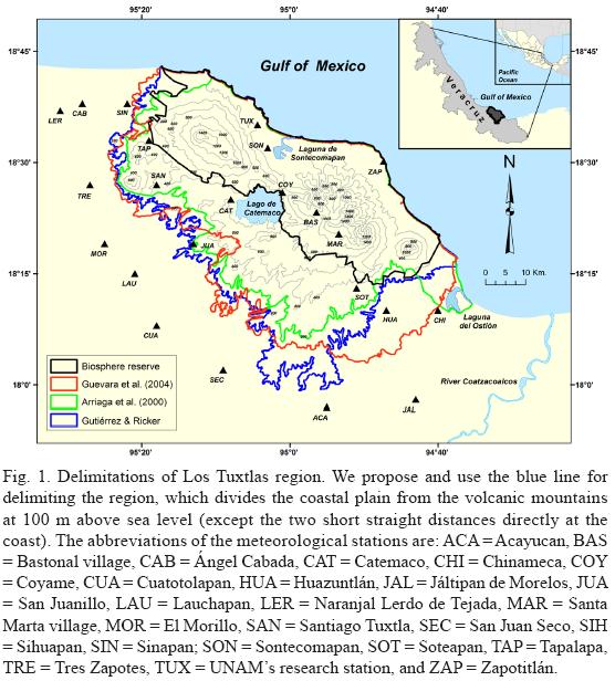
1. Guevara et al. (2004) in their book propose the delimitation shown in red in Figure 1 for the Sierra de Los Tuxtlas (Los Tuxtlas mountain range). These limits go back to maps elaborated by the Secretaría de Desarrollo Social (SEDESOL) of the federal government over 15 years ago. They calculate an extension of 329 941 hectares, but the exact criteria for choosing these limits are unclear.
2. In 1998, the Mexican government declared about half of the region (155 122 hectares) an UNESCO MAB Biosphere Reserve (SEMARNAP, 1998; Laborde, 2004). This delimitation is shown in black in Figure 1.
3. Arriaga-Cabrera et al. (2000) presented Los Tuxtlas region as a priority region for biological conservation, shown in green in Figure 1. They included the biosphere reserve, but extended the area in SW direction to include all land with at least 200 m above sea level (except at the coast). Furthermore, in SE direction the area was extended to include the Laguna del Ostión, near the city of Coatzacoalcos. Taking the corresponding shape file from the CONABIO map library (http://conabioweb.conabio.gob.mx/metacarto/metadatos.pl), we calculated 263 505 hectares for this polygon's area.
None of these delimitations is completely satisfying from a geographical viewpoint. They coincide only in that Los Tuxtlas region starts at the Gulf coast. We establish here a new, topographically more coherent delimitation, in blue in Figure 1, which also starts at the Gulf coast in NE direction, but has its limit at 100 m above sea level in SW direction. There is only a short distance towards north (with a length of 2308 m) and a small distance (2916 m length) towards east, where we connect the 100-m-contour line with the coast. This 100 m contour line was created from a digital elevation model, the hole-filled Shuttle Radar Topography Mission (SRTM, version 4) with a resolution of 90 meters, obtained from CGIAR-CSI SRTM 90 m database (available at http://srtm.csi.cgiar.org) (Jarvis et al., 2008). The region defined in this way has an area of 315 525 hectares, 96% of the area defined by Guevara et al. (2004). When oriented with an azimuth of 149.5°, the area can be put into a minimized rectangular of 89.1 km length and 55.9 km width. The biosphere reserve is included completely, representing 49% of our area. The priority area from Arriaga-Cabrera et al. (2000) represents 84% of our area, but includes outside of it the Laguna del Ostión.
Data sources
We employed eleven meteorological stations that we call principal stations, because they present a data record of at least 30 years (1977-2006) and are still collecting data (Table I). In addition, 13 auxiliary stations were added to elaborate interpolation maps for temperature and precipitation: Acayucan (abbreviated ACA, data record 1961-1980), Bastonal village (BAS, 1988-1989), El Morillo (MOR, 1956-1980), Huazuntlán (HUA, 1961-1980), Lauchapan (LAU, 1948-1989), Santiago Tuxtla (SAN, 1948-1986), Santa Marta (MAR, 1993-1997), San Juan Seco (SEC, 1956-1980), Sinapan (SIN, 1959-1980), Soteapan (SOT, 1976-1988), Tapalapa (TAP, 1956-1984), UNAM's Research Station (TUX, since 1971), and Zapotitlán (ZAP, 1925-1937). The station at San Andrés Tuxtla was not included, because it is only 8.8 km away from Santiago Tuxtla and not active anymore.
Thirteen of the 24 employed stations are within Los Tuxtlas area as defined by us, and eleven stations of Mexico's National Meteorological Service (Servicio Meteorológico Nacional) are near but outside Los Tuxtlas region. The latter were included to get a more complete data record, especially for the mapping. Another 10 meteorological stations close to the region of Los Tuxtlas were not employed (Cerrito, Garro, La Lima, Los Mangos, Mata de Limones, Juan Rodríguez Lara, San Juan Seco, Santa Elena, Santa Rosalía, and Zapotal), because they had either a very short climate record or were close to other stations with better climate data.
The data up to 2006 of 20 stations that report to Mexico's meteorological service were provided directly from this institution in an Excel file in 2008. The monthly data from TUX were provided directly by UNAM's research station. The average annual precipitation and average annual mean temperature for MAR, ZAP, and BAS are reported in Ramírez (1999).
Figure 1 shows the geographical distribution of the stations used in our study. Considering both principal and auxiliary stations, there are seven stations of Mexico's meteorological service within the region of Los Tuxtlas (CAT, COY, JUA, SAN, SON, SOT, TAP). Since the total Los Tuxtlas region considered here covers 315 525 hectares, each of the seven stations within the region covers on average an area of 45 075 hectares. This is 1.2-times larger, but still similar, to the average area of 37 519 hectares per meteorological station for all of Mexico. The latter number was calculated as Mexico's total area of 1945 748 km2 (including inland water bodies but without Guadalupe island) divided by 5186 stations reported by Quintas (2000).
The most problematic aspect of the distribution of meteorological stations Los Tuxtlas region is the lack of stations and consequently climate records on higher elevation. The eleven principal stations cover an elevational gradient from 19 to 338 m above sea level (Table I), while the peaks of the Santa Marta and San Martín Tuxtla volcanoes reach 1720 and 1680 m, respectively. The station SOT with a 14-year record is located at 430 m above sea level. For the region above 430 m, which represents 36.3% of the whole study area, there is only the two-year data of BAS at 1000 m above sea level, and the five-year data of MAR at 1200 m above sea level.
Definition of climatic variables for this study
Climate variables are not always consistently named. In addition, the averaging of means frequently causes confusion about what a variable really refers to, so it helps to list our definitions. The meteorological stations measured daily minimum temperature, daily maximum temperature, and daily precipitation, but provided us directly with the corresponding monthly values for precipitation and temperature. For this article we define and use the following climate variables that are calculated from these three original variables. Let Xbe any month from January to December, Y any year, and Y1 and Y2 any two distinct years:
1. Monthly minimum or maximum temperature (of month X in year Y): The average of the daily minimum temperature or the daily maximum temperature of all days of a specified month.
2. Monthly mean temperature (of month X in year Y) = (Monthly minimum temperature + Monthly maximum temperature)/2, of a specified month.
3. Average monthly minimum, mean, or maximum temperature (of month X during years from Y1 to Y2): The minimum, mean, or maximum temperature of a specified month, averaged over a specified period of years.
4. Annual minimum, mean, or maximum temperature (of year Y): The average of the monthly minimum, mean, or maximum temperature of all twelve months of a specified year. Note that this is approximately the same as averaging the daily temperatures of all days of the year (it is not exact, because the months differ in their number of days).
5. Average annual minimum, mean, or maximum temperature (during years Y1 to Y2): The annual minimum, mean, or maximum temperature, averaged over a specified period of years. Note that in Table II we report in addition the median annual mean temperature.
6. Monthly precipitation (of month X in year Y): The sum of daily precipitation for all days of a specified month.
7. Average monthly precipitation (of month X during years from Y1 to Y2): The monthly precipitation of a specified month, averaged over a specified period of years.
8. Annual precipitation (of year Y): The sum of daily precipitation for all days of a specified year, or alternatively the sum of monthly precipitation for all twelve months of a specified year.
9. Average annual precipitation (during yearsY1 to Y2): The annual precipitation, averaged over a specified period of years. Note that in Table III we report in addition the median annual precipitation.
Imputation of missing values, and correction of outliers and inhomogeneities
Most meteorological stations presented some missing data. The total percentages of missing data of the principal stations were 7.5 and 8.2% for monthly temperature and precipitation, respectively, during their overall recording period (Table I). Missing values of auxiliary stations were not estimated. For auxiliary stations (employed only in the spatial inter and extrapolation), the average monthly mean temperatures and average monthly precipitations were calculated with the available data.
Missing temperature values were estimated with the meteorological routine (MET) of the Dendrochronological Program Library (DPL) software, available at www.ltrr.arizona.edu/software.html. The algorithm uses the data from three surrounding stations whose data are most correlated with the data of the station with the missing value. The method is described briefly in Girardin et al. (2004). This procedure yields similar results as averaging three station values after correcting each value for the difference in elevation by a fixed lapse rate of 6 °C per 1000 m. Missing precipitation values of the principal stations were estimated in Excel with the normal ratio method (Paulhus and Kohler, 1952).
Subsequently, all monthly data records of the principal stations went through a quality control process to detect outliers and inhomogeneities, employing the software ProClimDB (Processing Climatological Data Bases), developed and provided by Petr Štepánek (www.climahom.eu/ProcData.html). The methods to detect outliers and inhomogeneities are explained in the software manual by Štepánek (2008), as well as for example in González-Hidalgo et al. (2009). ProClimDB creates reference series by comparing data values to values of those neighboring stations with the most correlated data, with the restriction that the mean Pearson correlation of all months has to be at least 0.5. Reference series are used for detection as well as correction of outliers and inhomogeneities. For homogeneity analysis, ProClimDB employs the complementary software AnClim (Štepánek, 2007; www.climahom.eu/AnClim.html), which applies the standard normal homogeneity test (SNHT) of Alexandersson (1986).
Figure 2 shows graphically the change from the raw data set to the corrected data set for the 11 principal stations (for 1959 or later, to 2006). A total of 616 outliers (3.3% of all records) were corrected in the time series of monthly precipitation, monthly maximum and minimum temperature (from which annual mean temperature is calculated). There was a higher number of outliers in the precipitation data (358 outliers), than in the data of maximum and minimum temperature (146 and 112, respectively). In the subsequent analyses, there were 86 inhomogeneities in the data of minimum temperature and 63 of maximum temperature. In the case of annual precipitation, there were only six inhomogeneities.
Further statistical analyses
Descriptive statistics for Tables II and III were calculated with Mathematica 8.0.1 (http://www. wolfram.com/products/mathematica/index.html). A small Mathematica notebook was programmed for that purpose. For calculating statistically significant deviation from a normal distribution, we employed the test from D'Agostino et al. (1990). This omnibus test for checking normality is easy to understand, due to its combined testing of skewness (asymmetry) and kurtosis (deviation from bell-shape) of the data distribution. Multiple linear regression was carried out with S-Plus 8.0. Exact probabilities of t-values were calculated with Mathematica.
Interpolation to develop maps of annual mean temperature and annual precipitation
We used spatial interpolation and extrapolation methods with the software ANUSPLIN to produce the two climate maps in Figures 3 and 4 for the complete region of Los Tuxtlas (ANU standing for Australian National University, and SPLIN for spline modeling). ANUSPLIN is a package of program modules developed for fitting surfaces of noisy data as functions of independent spline variables, as well as of parametric, linear sub-models, called covariates (Hutchinson, 2004). Originally it focused on climate interpolation (e.g., Hutchinson, 1995), though it is not restricted to that application. ANUSPLIN employs thin-plate smoothing splines, a method developed originally by Wahba (1979) and later modified for larger datasets by Bates and Wahba (1982). The method can be viewed as a generalization of standard multivariate linear regression. Details about the algorithms are found in the user guide (Hutchinson, 2004). ANUSPLIN has been used in many studies from regional to global scales (Hartkamp et al., 1999; Price et al., 2000; Jeffrey etal., 2001; Hijmans et al., 2005). In a recent study, Hutchinson et al. (2009) provide evidence that thin-plate smoothing spline employed in ANUSPLIN results in higher accuracy, compared with other methods such as DAYMET, GIDS, inverse distance interpolation, and ordinary kriging. For more information about the software see http://fennerschool.anu.edu.au/publications/ software/anusplin.php.
The simplest model consists in having climate data points that are georeferenced with latitude and longitude. ANUSPLIN subsequently models an interpolation surface among all climate data points, thus predicting the climatic variable in between the original points. A more sophisticated model consists in adding data from additional explanatory variables (covariates) to these georeferenced climate points in form of complementary raster layers. ANUSPLIN then predicts the climatic variable in between and possibly beyond the original data points (Hutchinson, 1998b; Joubert, 2007). For calculating here the layers of independent variables at a resolution of 90 m, the already mentioned hole-filled Shuttle Radar Topography Mission (see page 350) provided the digital elevation model. We modeled average annual mean temperature and average annual precipitation (each variable as a single, annual layer in ANUSPLIN, rather than twelve monthly layers).
For the interpolation map of average annual mean temperature, the independent variables were latitude and longitude, while elevation was a covariate. ANUSPLIN models the dependence of temperature as an approximately linear function of elevation. Extrapolation of predicted temperature to elevations over 1200 m sea level, where no meteorological stations existed, is carried out automatically by ANUSPLIN with an empirical temperature lapse rate, calculated with the input data.
For the interpolation map of average annual precipitation, the independent variables were latitude and longitude, while elevation, distance to the sea, the terrain's slope, and the terrain's aspect (cardinal direction) were used as covariates. Hastenrath (1967) showed for Central America that precipitation is generally highest at elevations around 1000 m above sea level, with lower values below and above that elevation. We hypothesize that such a pattern is also present in Los Tuxtlas region. Indirect evidence consists of the observed vegetation patterns. Limited direct evidence consists of the highest average annual precipitation having been measured at Bastonal village at 1000 m above sea level (BAS; 7824 mm, measured over two years), with a lower value measured again at Santa Marta village at 1200 m (MAR, 5085 mm, five years). ANUSPLIN has no special option to model this pattern; therefore we modified the digital elevation model in the following way: up to 1000 m, ANUSPLIN modeled increasing precipitation with increasing elevation by default, based on the variation provided with the input data. Above 1000 m, the digital elevation model that we provided as input to ANUSPLIN was inverted, as if the elevation would be decreasing again. ANUSPLIN thus automatically modeled above 1000 m decreasing precipitation with increasing elevation (up to 1720 m for the peak of the Santa Marta volcano). The area that falls under this hypothesis (above 1000 m), however, represents only 4.3% of the whole Los Tuxtlas region.
For the interpolation maps, the annual data of 22 principal and auxiliary meteorological stations were employed. The meteorological station at Sihuapan (SIH) was excluded, due to its proximity to the stations in Santiago Tuxtla (SAN) and Catemaco (CAT). The data from Bastonal village (BAS) also was not included in the interpolation, because its high precipitation is channeled via a valley-type landscape a long distance from the sea, a phenomenon not taken into account adequately by ANUSPLIN. The average distance among the 22 stations in the interpolation maps is 46 km, in a range from 6 to 111 km (n = 231 pairwise distances).
The distance to the Gulf of Mexico coast for each meteorological station was calculated employing the point distance routine in ARCGIS 9.3. It ranges from 0.2 to 60 km for the meteorological stations, and up to 85 km for the whole region. Precipitation is entering Los Tuxtlas region mainly from the ocean in the north and northeast. The effect of the terrain's slope and the terrain's aspect on orographic precipitation was modeled with a hillshade layer, employing the Hillshade routine of the ARCGIS's spatial analyst extension. This tool obtains the hypothetical illumination of a surface by determining illumination values for each cell in a raster, when setting a position for a hypothetical light source. Here, the shades do not refer to light shade but to rain shade. There are four input parameters needed for calculating the shade values in ARCGIS: 1) the angular direction As of the sun or source of rain, measured clockwise from 0 to 360° (azimuth); 2) the location of the source above the horizon, expressed as the angle Hs, with values that go from 0° at the horizon to 90° overhead; 3) the slope Hf, measured from 0° to 90°; and 4) the aspect Af, measured from 0° to 360°. The formula to calculate the relative radiance (or non-shade) Rf of each raster cell is: Rf = cos(Af - As) x sin Hf x cos Hs + cos Hf x sin Hs. The values of Rf range from 0 to 1, and are subsequently multiplied with 255 to widen the scale and obtain the so-called hillshade illumination value (Chang, 2009). We used A = 360° and Hs = 5°, while the slopes and aspects were calculated automatically from the digital elevation model. The use of the 5° angle created a hillshade surface with exposed windward slopes in the north and rain-shadows behind the mountain belt in the south. The inclusion of distance to the sea as a covariate for explaining variation in precipitation was confirmed with a Pearson correlation analysis. There was a significant correlation between average annual precipitation and the distance to the sea of the meteorological stations (r = -0.473, probability = 0.017, n = 22). The same was true between average annual precipitation and the two predictor variables hillshade value (r = 0.779, probability = 0.0001) and elevation (r = 0.695, probability = 0.0001). In contrast, average annual mean temperature was not significantly correlated with the two predictor variables, but only with elevation (r = -0.704, probability = 0.0001). For generating our final ANUSPLIN model, we explored second versus third spline orders, and the root square versus logarithmic transformation of the climate variable.
3. Results and discussion
Tables II and III show the descriptive statistics for annual mean temperatures and annual precipitation for each of eleven principal stations in the period 1977-2006. Following international standards for climate normals (Linacre, 1992), we used a 30-year period. There are obvious differences among the eleven meteorological stations. The meteorological stations with the lowest average annual mean temperature in Table II are Catemaco (CAT) and Coyame (COY) with 24.1°C, the one with the highest is Chinameca (CHI) with 27.2 "C.The meteorological station with the lowest average annual precipitation in Table III is Cuatotolapan (CUA) with 1272 mm, the one with the highest is Coyame (COY) with 4201 mm. The differences in precipitation depend mostly on the distance of the eleven stations to the sea, and their position on the windward or leeward side of the mountains. The inter-annual coefficients of variation of the average annual precipitation of the eleven stations range from 15.8% (COY) to 23.1% (TRE). These values indicate moderate inter-annual variability of precipitation in the region, compared with arid regions of North Mexico, where coefficients of variation can be as high as 50% (García, 1970).
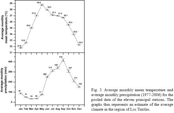
Table IV presents averages and standard errors of monthly mean temperature, and Table V of monthly precipitation for each month of the year of the eleven principal stations. Walter-Lieth climate diagrams are shown in Figure 5 for each station, to visualize the climatic differences within Los Tuxtlas (Walter and Lieth, 1960). The average monthly mean temperatures are plotted together with the average monthly precipitation on a scale, where 10 °C correspond to 20 mm, up to 100 mm precipitation. Above 100 mm, 1 °C corresponds to 20 mm precipitation. Humid periods are defined by precipitation curves above temperature curves; they are marked by vertical hatching up to 100 mm, and in black as wet periods above 100 mm of precipitation. Arid periods are defined by precipitation curves below temperature curves, and they are emphasized by dotting. Note in the graphs the midsummer drought ("canícula" or "veranillo") in July to August in some stations (CAB, CAT, SIH, TRE); it is not really a drought but just a small drop in precipitation for about a month (Magaña et al., 1999).
Pooling the monthly data of the eleven stations, Figure 6 presents the average monthly mean temperature and the average monthly precipitation. The coldest month in Los Tuxtlas on average is January (21.8 °C), the hottest month is May (28.8 °C). The driest month on average is March (34 mm), the wettest is September (418 mm). This represents a considerable range of variation among months.
Interpolation maps of average annual mean temperature and average annual precipitation
High resolution maps (90 meters) of average mean annual temperature and average annual precipitation were created with the ANUSPLIN software (Figs. 3 and 4). The final interpolation model for temperature employed second-order splines without transformation. The final model for precipitation employed third-order splines, the square-root transformation of precipitation (recommended by Hutchinson, 1998a), the elevation scaled to kilometers, and the hillshade values logarithmically transformed (Ln [X + 1]). The chosen models and transformations showed the best signal values, as well as the lowest values of the square root of generalized cross validation (RTGCV) and square root of the true mean square error (RTMSE). Standard errors of the covariates' coefficients could not be calculated, and consequently coefficients could not be interpreted statistically, because our data of two auxiliary stations (MAR, ZAP) consisted only of mean values.
The signal refers to the effective degrees of freedom of the model. The signal should not be greater than about half the number of data point; signals larger than this are indicative of either insufficient data points or short-range correlation in the data values (Hutchinson, 1998a). The signal was 8.6 for the temperature map and 10.4 for the precipitation map, which indicates that 22 data points are sufficient. The RTGCV is a conservative estimate of the overall standard prediction error of the interpolation. The RTGCV is based on the generalized cross validation (GCV), the latter being an estimate of the interpolation error obtained by removing each data point in turn, and fitting a spline surface to the remaining data, to evaluate how well each omitted point can be predicted. The square root of generalized cross validation of the final models was 0.67 °C for the temperature map, and 468 mm for the precipitation map.
A true estimator of the interpolation error is the square root of the true mean square error, which is a prediction of the standard error after the predicted data error has been removed (Hutchinson, 2004). The RTMSE of the final models were 0.33 °C for the temperature map, and 233 mm for the precipitation map. Dividing in the case of the precipitation map the RTMSE by the mean values for the whole interpolation surface results in the estimated predictive error, being here 9.4% (233 /2474). Calculating the error as a proportion of the mean is not sensible for temperature, because temperature in degrees Celsius has an essentially arbitrary cero point. Hutchinson (2004) mentions that RTMSE of 0.5 °C are typical when fitting splines to temperature data, and predictive errors of 10% are typical for surfaces fitted to precipitation data. Finally, we tested the distributions of the residuals at the points of meteorological stations (n = 22) in both maps. They do not deviate from a normal distribution (with D'Agostino's and Shapiro-Wilk's tests).
Hutchinson (1998a) and Joubert (2007), for example, have modeled topography, and report rainfall interpolation with varying topography to be challenging. In our study, the strong rain-shadow effect, with a precipitation difference of about 3000 mm over a distance of 10 km between the leeward and the windward sides of the San Martín Tuxtla volcano could be captured accurately by modeling it as a hillshade, and by taking into account the distance to the sea. In addition, our study apparently is the first one where the nonlinear pattern of precipitation as a function of elevation, with maximum precipitation at around 1000 m above sea level, is modeled successfully with ANUSPLIN.
As explained in the methods, the two-year data from BAS was not included in the interpolation, where it is predicted to receive 6281mm (80.3% of the measured value). The underestimation in the model is due to the relatively large distance of BAS to the sea, while in reality precipitation is channeled to BAS via a valley-type landscape from the sea. The predicted annual mean temperature at BAS is 20.9 °C, the measured one is 22.0 °C.
The fact that the measured value of 7824 mm at BAS exceeds the maximum predicted value of 7748 mm for any point on the map (Fig. 4) gives us confidence in the predicted results of the extrapolation with ANUSPLIN. The predicted average annual mean temperature of 17.4 °C at an elevation of about 1700 m above sea level (Fig. 3) seems also reasonable (Soto and Gama, 1997), though there is no data for confirmation.
If validated with more measurement years, the annual average precipitation at BAS would be the highest record in Mexico, and indeed falls among the extreme values worldwide. The highest average annual precipitation reported by Mexico's Servicio Meteorológico Nacional is 6096 mm for a period of 14 years at the Campamento Vista Hermosa, located in the state of Oaxaca (17.40N; 96.18W; 1000 m above sea level). The world's wettest regions are considered to be in the Chocó in western Colombia, with 12 700 mm (measured from 1952 to 1960; Poveda and Mesa, 2000), and Cherrapunjee in northeastern India with 11 987 mm (1973-2003; Murata etal., 2007). The maximum rainfall in Cherrapunjee for a single year was even 24 555 mm (in 1974).
Currently, the maps of Figures 3 and 4 are the most detailed ones available for the region of Los Tuxtlas. A database that is often used in large-scale climate modeling (including in Mexico) is WorldClim, a set of global climate layers (climate grids) with a spatial resolution of one square kilometer (http://www.worldclim.org/). Interpolation forWorldClim has also been carried out with ANUSPLIN, but only employing longitude, latitude, and elevation (Hijmans et al., 2005). Our spatial climate models, represented in the maps of Figures 3 and 4, reveals major improvements when compared to spatial climate data from WorldClim for the region of Los Tuxtlas:
1. The spatial resolution is improved in our maps from 1 km in WorldClim to 90 m.
2. WorldClim predicts a range of average annual precipitation from 1420 to 3710 mm, which is too small. The maximum value is only 88% of the measured average annual precipitation in Coyame (COY; 4201 mm), and 48% of the maximum value predicted in our map (Fig. 4; 7748 mm). The range of average annual mean temperature in WorldClim is 16.8 to 25.9 °C, similar to our predicted range of 17.4 to 26.3 °C (Fig. 3).
3. Different from the expected pattern, WorldClim predicts the wettest areas mainly in the lowlands at the coast, and to a lesser extent on the peaks of the three volcanoes. The spatial distribution of the predicted average mean temperature map in WorldClim, however, is similar to ours in Fig. 3.
The information about temperature and precipitation in Figures 3 and 4 makes it possible to derive directly Holdridge forest (life) zones (Holdridge, 1947; Holdridge et al., 1971). The revealed spatial patterns of forest life zones in Figure 7 are especially useful for further floristic research in Los Tuxtlas region. In Holdridge's Diagram for the classification of world life zones, forest zones are determined as a function of average annual mean temperature and average annual precipitation, as well as latitude and elevation. For Los Tuxtlas region, the areas with an average annual mean temperature above 24 °C and below 2000 mm precipitation correspond to tropical lowland dry forest, from 2000 to 4000 mm to tropical lowland moist forest, and from 4000 to the maximum projected precipitation to tropical lowland wet forest. The term "lowland" is not used in the original classification by Holdridge, but it is convenient to distinguish lowland forest from premontane forests that are found in the Holdridge system at higher elevations, where the average annual mean temperature is below 24 °C. For premontane forests, the precipitation criteria change. From 1500 to 3000 mm the life zone is called tropical premontane moist forest, from 3000 to 6000 mm tropical premontane wet forest, and above 6000 mm tropical premontane rain forest. Note that the term "rain forest" in the Holdridge sense is very narrow in its definition, applying only to forests in regions with extremely high precipitation. In contrast, Malhi and Wright (2004) calculate that the global average annual precipitation in what they call tropical rainforest regions is 2180 mm (and the average annual mean temperature is 25.4 °C). Translated back into the Holdridge system, this corresponds to tropical lowland moist forest, with the precipitation being barely higher than the limit for tropical lowland dry forest.
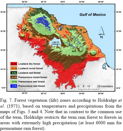
Figure 7 gives also the percentages for the relative extension of each of the six forest life zones in the region of Los Tuxtlas. The most extensive life zone is the lowland dry forest with 26.9%, mainly in the southern part of the region. Premontane wet forest follows with 22.5%, and then premontane moist forest (21.4%) and lowland moist forest (21.1%). There is no true lowland rain forest in the Holdridge sense, which would require an average annual precipitation of at least 8000 mm. There is, however, an extension of 3.1% premontane rain forest, distributed on the slopes of the three volcanoes, where the precipitation at higher elevations is at least 6000 mm.
Analysis of climate change
We tested if global climate change can be detected in Los Tuxtlas with a time series of 48 years from 1959 to 2006. The tested variables were the annual mean temperature and the annual precipitation, respectively. Statistical modeling of time series data frequently presents autocorrelated (or serially correlated) error terms, meaning that the error term ut at time t is correlated with error terms ut_u ut_2... and ut+1, ut+2... . Such correlation in the error terms often arises from the correlation of the omitted variables that the error term captures (Maddala and Lahiri, 2009). Using the generalized least squares (GLS) estimator in regression models with time series error terms is recommended in Box et al. (2008). Using ordinary least squares (OLS) regression for time series can be inefficient; e.g., Safi (2008) presents an example with serially correlated data, where the OLS standard error is about 71% bigger than its GLS competitor, though in other examples the OLS may also perform reasonably well.
To test a relatively long, yet balanced data set, seven of our principal stations with a complete data record from 1959 to 2006 (48 years) were used in this analysis (CAB, CAT, COY, CUA, LER, JUA,TRE). Our final regression model was the following: (Annual mean temperature) or (Annual precipitation) = b0 + b1 x Year + b2 x Station, where the variable "Station" was converted from a nominal to a continuous variable by replacing the station name with its average value of temperature or precipitation for 1959-2006. An interaction term (b3 x Year x Station) was also tested, but turned out to be non-significant and destabilizing the coefficients. Table VI shows the resulting statistical parameters of the regression analysis, and Figures 8 and 9 the corresponding partial residual plots, leading to the following conclusions:
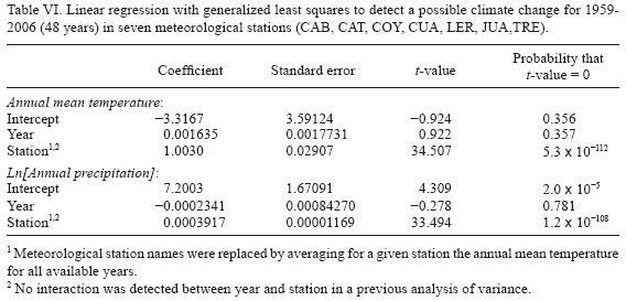
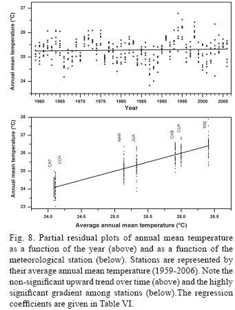
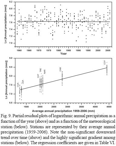
1. There are statistically highly significant differences among meteorological stations in both annual mean temperature and annual precipitation.
2. There is no statistically significant increase of mean annual temperature detectable for the seven stations over the 48 years. There is, however, a non-significant trend of increasing temperature of 0.016 °C per decade (0.001635 °C/year x 10 years/decade). This trend is 16-times lower than the mean warming rate of 0.26 °C per decade since the mid-1970s, reported for tropical rain (or moist) forests worldwide by Malhi and Wright (2004).
3. There is no statistically significant change of annual precipitation detectable over the 48 years. There is, however, a non-significant trend of decreasing precipitation of 0.23% less precipitation per decade (1 - e-0002341 x 10).
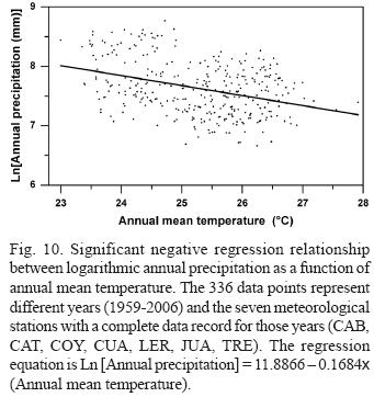
4. Are such opposite effects of decreasing precipitation with increasing temperature expected? A regression analysis of annual mean temperature as a function of annual precipitation in Figure 10 indicates that it is expected. The negative slope of -0.1684 is highly significant. According to this relationship, the expected decrease in precipitation from a 0.016 °C increase in temperature is 0.27% (1 - e-0.1684x 0.0016x10), similar directly calculated downward trend of 0.23%.
Global Climate change is not a uniform phenomenon worldwide, but presents considerable variations of temperature and precipitation changes, as a function of the time period and the region (Trenberth and Jones, 2007; Easterling and Wehner, 2009). On average, tropical rain (or moist) forests worldwide experienced warming at a mean rate of 0.26 °C per decade since the mid-1970s, while precipitation during 1960-1998 has declined for example in Africa, but not in Amazonia (Malhi and Wright, 2004). No significant net change for precipitation since the 1920 is also reported by Satyamurty et al. (2010) for Brazilian Amazonia. Pavia et al. (2009) reported that Mexico on average cooled down during 1940-1969, and warmed up 1970-2004; notably, even during the warming period, 46 stations (17%) out of 267 Mexican stations had a negative trend in maximum surface air temperature. In this context it is conceivable that no significant changes in temperature and precipitation have occurred in Los Tuxtlas.
Trenberth et al. (2003) state that from 1973 to 1995 there have been significant increases of 2-3% per decade in relative humidities over the Caribbean, and upward trends in precipitable water also in other regions worldwide. A general temperature increase automatically increases the water-holding capacity of the atmosphere. Rain drops, however, carry less temperature from higher altitudes to the ground (Anderson etal., 1998), and cause surface evaporative cooling (Dai etal., 1997). Furthermore, clouds have a damping effect on the diurnal temperature range, aiding cooling of the Earth's surface (Dai et al., 1997). In consequence, people in hot regions generally experience that the temperature drops when it rains. One could hypothesize the existence of a damping feedback mechanism: increasing temperature leads to increasing precipitation, which leads to buffering the temperature increase; this in turn could inhibit the precipitation increase again. At the end, little climate change would occur in such a situation, as observed in our study for the region of Los Tuxtlas. The energy, however, contained in increased temperature would possibly be transferred into an accelerated cycling of the water through the atmosphere. Ultimately the effect predicted by Trenberth (2011) would be observed: "It never rains but it pours!"
4. Conclusions
Los Tuxtlas is a Mexican tropical region at the Gulf of Mexico, with an elevational gradient from sea level to 1720 m on an otherwise relatively flat coastal plateau. There are two climates according to Koppen's climatic classification: humid tropical (type A) at low and middle elevations, and moist with mild winters (type C) at high elevations. We propose here a new delimitation for the region of Los Tuxtlas, taking the 100 m-contour line as the region's limit, except for the coast. The extension of Los Tuxtlas region is 315 525 hectares, including a 155 122-hectare biosphere reserve. Our study, based on data from 24 meteorological stations with varying data records between 1925 and 2006, leads to the following conclusions:
1. Among eleven stations, the average annual mean temperature varied from 24.1 to 27.2 °C, and the average annual precipitation from 1272 to 4201 mm, during the 30-year period 1977-2006. Additional measurements indicate locations with over 7000 mm average annual precipitation at higher elevations, which would be among the highest recorded in Mexico. Based on this data and a spatial inter and extrapolation model (ANUSPLIN), we present two new climate maps for the region of Los Tuxtlas, one for average annual mean temperature and the other for average annual precipitation. In addition, we present a map of climate-based forest life zones according to Holdridge's classification.
2. Pooling the data of the eleven stations and the 30 years, the coldest month in Los Tuxtlas on average is January (21.8 °C), the hottest month is May (28.8 °C). The driest month on average is March (34 mm), the wettest is September (418 mm).
3. To analyze the time series of temperature and precipitation over 48 years, we employed linear regression with generalized least squares. There are no statistically significant changes of annual mean temperature or annual precipitation, but a low upward trend of 0.016 °C per decade in temperature, and a low downward trend of -0.23% per decade in precipitation. We show that such an opposite change between temperature and precipitation is expected.
Finally, we present one possible explanation why a temperature increase might not have happened in Los Tuxtlas region.
Acknowledgements
We thank the Posgrado en Ciencias Biológicas of the Universidad Nacional Autónoma de Mexico (UNAM) for supporting the first author's doctoral thesis project, including a scholarship from the Consejo Nacional de Ciencia y Tecnología (CONACyT). Furthermore, the Programa de Apoyo a Proyectos de Investigación e Innovación Tecnológica (PAPIIT) of UNAM provided financial support to carry out the project IN217008 "La relación entre crecimiento y clima en árboles tropicales: un estudio dendrocronológico en la selva de Los Tuxtlas, Veracruz", which included the presented research. We are grateful to Alejandro González-Serratos of Mexico's Servicio Meteorológico Nacional in Mexico City for providing the climate data from 20 meteorological stations, to Rosamond Coates (Instituto de Biología, UNAM) for providing the climate data from UNAM's research station (TUX), and to Gabriel Díaz Padilla of the Instituto Nacional de Investigaciones Forestales, Agrícolas y Pecuarias (INIFAP) in Xalapa on his advice on elaborating interpolation maps with the software ANUSPLIN. Petr Štepánek (Czech Hydrometeorological Institute, Brno, Czech Republic) kindly provided the software ProClimDB, and gave valuable advice on how to use it. Finally, we thank Juan Núñez-Farfán (Instituto de Ecología, UNAM) and Miguel Martínez-Ramos (Centro de Investigaciones en Ecosistemas, UNAM) for their participation in the first author's doctoral committee.
References
Alexandersson H., 1986. Ahomogeneity test applied to precipitation data. Int.J. Climatol. 6,661-675. [ Links ]
Anderson S. P., A. Hinton and R. A. Weller, 1998. Moored observations of precipitation temperature. J. Atmos. Ocean. Tech. 15, 979-986. [ Links ]
Arriaga-Cabrera L., J. M. Espinoza, C. Aguilar-Zúñiga, E. Martínez-Romero, L. Gómez-Mendoza and E. Loa-Loza (coordinadores), 2000. Regiones terrestres prioritarias de Mexico. Comisión Nacional para el Conocimiento y Uso de la Biodiversidad (CONABIO), Mexico D. F., Mexico, 609 pp. [ Links ]
Bates D. and G. Wahba, 1982. Computational methods for generalised cross validation with large data sets. In: Treatment of integral equations by numerical methods (C. T. H. Baker and G. F. Miller, Eds.). Academic Press, New York, USA, 283-296. [ Links ]
Box G. E. P., G. M. Jenkins and G. C. Reinsel, 2008. Time series analysis: Forecasting and control. 4th Ed. John Wiley & Sons, Hoboken, New Jersey, USA, 784 pp. [ Links ]
Castillo-Campos G. and J. Laborde, 2004. Vegetación. In: Los Tuxtlas: el paisaje de la sierra (S. Guevara, J. Laborde and G. Sánchez-Ríos, Eds.). Instituto de Ecología A.C., Xalapa, Veracruz, Mexico, 231-270. [ Links ]
CETENAL, 1970. Carta de climas, hoja Coatzacoalcos, escala 1:500 000. Comisión de Estudios del Territorio Nacional. Secretaría de la Presidencia, Mexico D. F., Mexico. [ Links ]
Chang K., 2009. Introduction to geographic information systems. 5th Ed. McGraw-Hill, Boston, USA, 448 pp. [ Links ]
D'Agostino R. B., A. Belanger and R. B. D'Agostino Jr., 1990. A suggestion for using powerful and informative tests of normality. Am. Stat. 44, 316-321. [ Links ]
Dai A., A. D. del Genio and I. Y. Fung, 1997. Clouds, precipitation and temperature range. Nature 386, 665-666. [ Links ]
Easterling D. R. and M. F. Wehner, 2009. Is the climate warming or cooling? Geophys. Res. Lett. 36, L08706.1-L8706.3. [ Links ]
García E., 1970. Los climas del estado de Veracruz. An. Inst. Bio. Serie Bot. 41, 3-42. [ Links ]
García E., 1973. Modificaciones al sistema de clasificación climática de Kóppen (para adaptarlo a las condiciones de la República Mexicana.) 2nd Ed. Universidad Nacional Autónoma de México, México D. F., Mexico, 246 pp. [ Links ]
Girardin M., J. Tardif, M. Flannigan and Y. Bergeron, 2004. Multicentury reconstruction of the Canadian Drought Code from eastern Canada and its relationship with paleoclimatic indices of atmospheric circulation. Clim. Dynam. 23, 99-115. [ Links ]
González C., 1991. Regionalización climática de la sierra de Santa Marta y el volcán San Martín Pajapan, Veracruz. Master's thesis. Facultad de Ciencias, Universidad Nacional Autónoma de México, México D. F., Mexico, 78 pp. [ Links ]
González-Hidalgo J. C., J.-A. López-Bustins, P. Stepánek, J. Martín-Vide and M. de Luis, 2009. Monthly precipitation trends on the Mediterranean fringe of the Iberian Peninsula during the second-half of the twentieth century (1951-2000). Int. J. Climatol. 29, 1415-1429. [ Links ]
Guevara S., J. Laborde and G. Sánchez-Ríos, 2004. Introducción. In: Los Tuxtlas: el paisaje de la sierra (S. Guevara, J. Laborde and G. Sánchez-Ríos, Eds.). Instituto de EcologíaA.C., Xalapa, Veracruz, Mexico, 18-27. [ Links ]
Hartkamp A., K. de Beurs, A. Stein and J. White, 1999. Interpolation techniques for climate variables. International Maize and Wheat Improvement Center (CIMMYT), Geographic Information Systems Series 99-01, México D. F., Mexico, 26 pp. [ Links ]
Hastenrath S., 1967. Rainfall distribution and regime in Central America. Theor. Appl. Climatol. 15, 201-241. [ Links ]
Hewitt C. and A. Jackson, 2003. Handbook of atmospheric science: Principles and applications. Wiley-Blackwell, Oxford, U.K., 648 pp. [ Links ]
Hijmans R., S. Cameron, J. Parra, P. Jones and A. Jarvis, 2005. Very high resolution interpolated climate surfaces for global land areas. Int. J. Climatol. 25, 1965-1978. [ Links ]
Holdridge L., 1947. Determination of world plant formations from simple climatic data. Science 105, 367-368. [ Links ]
Holdridge L., W. Grenke, W. Hatheway, T. Liang and J. Tosi, 1971. Forest environments in tropical life zones: A pilot study. Oxford Pergamon Press, Oxford, U.K., 747 pp. [ Links ]
Hutchinson M. F., 1995. Interpolating mean rainfall using thin plate smoothing splines. Int. J. Geogr. Inf. Sci. 9,385-403. [ Links ]
Hutchinson M. F., 1998a. Interpolation of rainfall data with thin plate smoothing splines. Part I: Two dimensional smoothing of data with short range correlation. J. Geogr. Inf. Dec. Anal. 2, 139-151. [ Links ]
Hutchinson M. F., 1998b. Interpolation of rainfall data with thin plate smoothing splines. Part II: Analysis of topographic dependence. J. Geogr. Inf. Dec. Anal. 2, 152-167. [ Links ]
Hutchinson M. F., 2004. ANUSPLIN Version 4.3 - User Guide. Centre for Resource and Environmental Studies, Australian National University, Canberra, Australia, 57 pp. [http:// fennerschool.anu.edu.au/publications/software/anusplin.php] [ Links ].
Hutchinson M. F., D. W. Mckenney, K. Lawrence, J. Pedlar, R. Hopkinson, E. Milewska, and P. Papadopol, 2009. Development and testing of Canada-wide interpolated spatial models of daily minimum/maximum temperature and precipitation for 1961-2003. J. Appl. Meteor. 48, 725-741. [ Links ]
Jarvis A., H. I. Reuter, A. Nelson and E. Guevara, 2008. Hole-filled SRTM for the globe, version 4, digital elevation model database available from the CGIAR-CSI SRTM (90 m). Available at: http://srtm.csi.cgiar.org (accessed in September 2009). [ Links ]
Jáuregui E., 1963. Wet-bulb temperature and discomfort index areal distribution in Mexico. Int. J. Biometeorol. 11, 21-28. [ Links ]
Jeffrey S., J. Carter, K. Moodie and A. Beswick, 2001. Using spatial interpolation to construct a comprehensive archive of Australian climate data. Environ. Modell. Softw. 16, 309-330. [ Links ]
Joubert S. J., 2007. High resolution climate variable generation for the Wester Cape. Master's thesis, University of Stellenbosch, Stellenbosch, South Africa, 96 pp. [ Links ]
Köppen W., 1936. Das Geographische System der Klimate. Handbuch der Klimatologie Vol 1. Gebrüder Bornträger, Berlin, Germany, 44 pp. [ Links ]
Laborde J., 2004. La Reserva de la Biosfera. In: Los Tuxtlas: el paisaje de la sierra (S. Guevara, J. Laborde and G. Sánchez-Ríos, Eds.). Instituto de Ecología A. C., Xalapa, Veracruz, Mexico, 271-281. [ Links ]
Linacre E., 1992. Climate data and resources: A reference and guide. Routledge, London, U.K., 366 pp. [ Links ]
Maddala G. S. and K. Lahiri, 2009. Introduction to econometrics. John Wiley & Sons, Chichester, West Sussex, U.K., 634 pp. [ Links ]
Magaña V., J. Amador and S. Medina, 1999. The midsummer drought over Mexico and Central America. J. Climate 12, 1577-1588. [ Links ]
Malhi Y. and J. Wright, 2004. Spatial patterns and recent trends in the climate of tropical rainforest regions. Philos. T. Roy. Soc. B. 359, 311-329. [ Links ]
Martín-del Pozzo A. L., 1997. Geologia. In: Historia natural de Los Tuxtlas (E. González-Soriano, R. Dirzo and R.C. Vogt, Eds.). Instituto de Biología, Universidad Nacional Autónoma de México, México D. F., Mexico, 25-31. [ Links ]
Murata F., T. Hayashi, J. Matsumoto and H. Asada. 2007. Rainfall on the Meghalaya plateau in northeastern India: One of the rainiest places in the world. Nat. Hazards 42, 391-399. [ Links ]
Paulhus J. L. H. and M. A. Kohler, 1952. Interpolation of missing precipitation records. Mon. Weather Rev. 80, 129-133. [ Links ]
Pavia E., F. Graef and J. Reyes, 2008. Annual and seasonal surface air temperature trends in Mexico. Int. J. Climatol. 29, 1324-1329. [ Links ]
Poveda G. and O. Mesa, 2000. On the existence of Lloró (the rainiest locality on earth): Enhanced ocean-land-atmosphere interaction by a low-level jet. Geoph. Res. Lett. 27, 1675-1678. [ Links ]
Price D., D. McKenney, I. Nalder, M. F. Hutchinson and J. Kesteven, 2000. A comparison of two statistical methods for spatial interpolation of Canadian monthly mean climate data. Agr. Forest Meteorol. 101,81-94. [ Links ]
Quintas I., 2000. ERIC II. Base de datos climatológica compactada, archivos y programa extractor (CD-ROM). Instituto Mexicano de Tecnología del Agua (IMTA), Comisión Nacional del Agua, Jiutepec, Morelos, Mexico,75 pp. [ Links ]
Ramírez F., 1999. Flora y vegetación de la Sierra de Santa Marta, Veracruz. Bachelor's thesis, Facultad de Ciencias, Universidad Nacional Autónoma de México, México D.F., Mexico, 409 pp. [ Links ]
Ricker M., E. López-Vega y P. Mendoza-Márquez. Crecimiento a largo plazo, densidad de la madera, y masa foliar específica de 18 especies arbóreas en la selva alta perennifolia de Los Tuxtlas (Veracruz, Mexico). In: Avances y perspectivas en la investigación de bosques tropicales y sus alrededores: Los Tuxtlas (V. H. Reynoso and R. Coates, Eds.). Instituto de Biología, Universidad Nacional Autónoma de México. Mexico D. F., Mexico. In press. [ Links ]
Safi S., 2008. The Efficiency of OLS in the presence of autocorrelated errors.VDM Verlag Dr. Müller, Saarbrücken, Germany, 140 pp. [ Links ]
Satyamurty P., A. A. de Castro, J. Tota, L. E. da Silva-Gularte and A. O. Manzi, 2010. Rainfall trends in the Brazilian Amazon Basin in the past eight decades. Theor. Appl. Climatol. 99, 139-148. [ Links ]
SEMARNAP, 1998. Decreto de Reserva de la Biosfera, la región de Los Tuxtlas. Secretaría del Medio Ambiente, Recursos Naturales y Pesca, 23 de noviembre. Diario Oficial de la Federación DXLII (16), México, 6-21. [ Links ]
Soto M., 1976. Algunos aspectos climáticos de la regiòn de Los Tuxtlas. In: Investigaciones sobre la regeneración de selvas altas en Veracruz, México (A. Gómez-Pompa, R.S. del Amo, C. Vázquez-Yanes and A. Butanda, Eds.). Compañía Editorial Continental S.A. (CECSA), México D.F., Mexico, 70-111. [ Links ]
Soto M. and L. Gama, 1997. Climas. In: Historia natural de Los Tuxtlas (E. González-Soriano, R. Dirzo and R. C. Vogt, Eds.). Instituto de Biología, Universidad Nacional Autónoma de México, México D.F., Mexico, 7-23. [ Links ]
Soto M., 2004. Clima. In: Los Tuxtlas: el paisaje de la sierra (S. Guevara, J. Laborde and G. Sánchez-Ríos, Eds.). Instituto de Ecología A. C., Xalapa, Veracruz, Mexico, 195-199. [ Links ]
Štepánek P., 2007. AnClim: Software for time series analysis. Department of Geography, Faculty of Natural Sciences, Masaryk University, Brno, Czech Republic, [http://www.climahom.eu/ AnClim.html] [ Links ].
Štepánek P., 2008. Documentation of ProclimDB: Software for processing climatological datasets. Department of Geography, Faculty of Natural Sciences, Masaryk University, Brno, Czech Republic [http://www.climahom.eu/ProcData.html] [ Links ].
Tejeda A., F. Acevedo and E. Jáuregui, 1989. Atlas climático del Estado de Veracruz. Universidad Veracruzana, Xalapa, Mexico, 150 pp. [ Links ]
Trenberth K. E., A. Dai, R.M. Rasmussen and D. B. Parsons, 2003. The changing character of precipitation. B. Am. Meteorol. Soc. 84, 1205-1217. [ Links ]
Trenberth K. E. and P. D. Jones, 2007. Observations: surface and atmospheric climate change. In: Climate Change 2007: The Physical Science Basis (S. Solomon, D. Qin, M. Manning, Z. Chen, K. B. M. Marquis, M. T. Averyt, and H. L. Miller, Eds.). Cambridge University Press, New York, USA, 235-336. [ Links ]
Trenberth, K. E. 2011. Changes in precipitation with climate change. Clim. Res. 47, 123-138. [ Links ]
Wahba G., 1979. How to smooth curves and surfaces with splines and cross-validation. In: Proceedings of the 24th Conference on the Design of Experiments, US Army Research Office 79-2, Research Triangle Park, North Carolina, USA, 167-192. [ Links ]
Walter H. and H. Lieth, 1960. Klimadiagramm-Weltatlas. G. Fischer, Jena, Germany, 150 pp. [ Links ]

