


Serviços Personalizados
Journal
Artigo
 Inglês (pdf)
 Artigo em XML
 Referências do artigo
 Enviar este artigo por email
Indicadores
-
 Citado por SciELO
 -
 Acessos
Links relacionados
-
 Similares em
SciELO
Similares em
SciELO
Compartilhar

 Permalink
Atmósfera
versão impressa ISSN 0187-6236
Atmósfera vol.23 no.4 Ciudad de México Out. 2010
Sea surface temperature and mixed layer depth changes due to cold–air outbreak in the Gulf of Mexico
E. E. VILLANUEVA, V. M. MENDOZA and J. ADEM
Centro de Ciencias de la Atmósfera, Universidad Nacional Autónoma de México.
Circuito Exterior, Ciudad Universitaria, México D.F. 04510, México.
Corresponding author: E. E. Villanueva; e–mail: eevu@atmosfera.unam.mx
Received December 10, 2009; Accepted July 27, 2010
RESUMEN
Se muestra el impacto de un frente frío o Norte en la capa de mezcla marina del Golfo de México (GoM) durante el periodo 18–23 de octubre de 1999. Un modelo numérico basado en la ecuación de la energía térmica y en la ecuación de balance entre la energía térmica y la energía mecánica, es usado para calcular los cambios en la temperatura de la superficie marina y los cambios en la profundidad de la capa de mezcla marina, debidos al forzamiento atmosférico producido antes y durante el frente frío en estudio. Se analiza la importancia de cada una de las diferentes contribuciones a la tendencia de la temperatura como son el forzamiento térmico en la superficie, la penetración vertical de agua fría desde la termoclina, el transporte horizontal de energía térmica por corrientes y turbulencia en la capa de mezcla. Durante el paso del frente frío los cambios en la temperatura de la superficie marina estuvieron marcadamente influenciados por el incremento en la rapidez del viento a nivel de superficie. Los experimentos mostraron que la penetración vertical de agua fría a través de la termoclina resultó ser el proceso determinante en el enfriamiento de la capa de mezcla, aún por encima de los flujos de calor latente y sensible y del transporte horizontal por corrientes oceánicas y por remolinos turbulentos.
ABSTRACT
The impact of a cold–air outbreak (CAO) on the mixed layer in the Gulf of México (GoM), during the period 18–23 October 1999, is shown in this work. A numerical model, based on the thermal energy equation and the balance equation between the thermal and mechanical energies, is used for computing both, the sea surface temperature (SST) and the sea mixed layer depth (MLD) changes due to atmospheric forcing before and during the CAO. The importance of the contributions to the temperature tendency by thermal forcing at the surface, the vertical entrainment of cold water from the thermocline, the horizontal transport of thermal energy by ocean currents and by turbulent eddies in the mixed layer are analyzed, as well as the contributions to the entrainment velocity by deepening of the mixed layer and the Ekman's pumping velocity. During the passage of the CAO on the GoM the SST changes were markedly influenced by the increase in the surface wind speed. At the end of the period the experiments show that the vertical entrainment turned out to be the most determining process in the cooling of the mixed layer, even overhead of the latent and sensible heat fluxes and the horizontal transport by ocean currents and by turbulent eddies.
Keywords: Sea surface temperature, mixed layer depth, cold–air outbreak, Gulf of México.
1. Introduction
The response from the ocean to changes in the atmospheric conditions has been studied mainly to identify the processes which determine the thermal structure in the mixed layer. O'Brien et al., (1977) as well as Niiler and Kraus (1977) performed a general review of the upper ocean models. Camp and Elsberry (1978) simulated the upper ocean response during strong forcing events by using a bulk turbulent kinetic energy model and suggested that the one–dimensional mixing processes play an important role in the deepening and cooling of the ocean mixed layer. However, when the ocean dynamics exert an important influence on the evolution of SST, particularly under severe storms, it is more convenient to study the dynamics from a single reduced–gravity model than from one–dimensional physics basis (Busalacchi and O'Brien, 1981). Schopf and Cane (1983) studied the interactions between the dynamics and mixed layer physics in the equatorial ocean applying a primitive equations model, in which the dynamics of mixed layer was parameterized in terms of the turbulent kinetic energy balance. Such model demonstrated that not only the surface heating is essential for the maintenance of the stratification at the equator, but that the vertical transfers of momentum and mixed layer entrainment must be included.
Local thermodynamic processes and turbulent mixing processes primarily determine the response of the SST to atmospheric forcing in the oceans. On the other hand, Price (1981) examined the open ocean's response to a steadily moving hurricane, emphasizing the response of the SST to the effects of processes such as upwelling, horizontal advection and pressure gradients. His primary goal was to interpret the decrease of SST taking place during the Eloise hurricane passage in the GoM, which seemed to cause a combination of heat loss and cold water's entrainment (vertical mixing) into the mixed layer, showing hence that the response is essentially a problem of dynamics of the mixed layer.
In smaller areas such as the Southern China Sea, the heat budget assessment indicates that although the surface heat flux is fundamental in the seasonal cycle of SST, the effect of the ocean dynamics is not negligible (Qu, 2001).
From October to March, the CAO events in the GoM are generally characterized by dry and cold air with intense winds that could reach 70 km/h. This dry and cold air often moves from high latitudes towards the continental south–eastern region of North America until it penetrates into the gulf. Nowlin and Parker (1974) developed the first surveys on the change in temperature–salinity relations of the waters in a shelf region of the north–western GoM, prior and following the passage of a frontal system from north to south across the gulf. They found that evaporation and sensible heat exchanges towards the atmosphere may lead to significant modification of water masses.
This paper presents a case study of changes in the SST, as well as changes in the mixed layer depth (MLD) due to the passage of a CAO through the GoM (October 18–23, 1999). The basic hypothesis states that in this region much of the oceanic response to strong forcing events can be simulated with the bulk turbulent kinetic energy models such as those implemented by Kraus and Turner (1967), and modified by Alexander and Woo Kim (1976), Bleck et al. (1989), Mendoza et al. (2005) and Villanueva et al. (2006). These mentioned scientists assumed that the SST changes in the mixed layer can be mainly attributed to the entrainment produced by transformation of potential energy into turbulent kinetic energy by convection in the layer additionally they also consider the role of the Ekman oceanic dynamics.
The paper is presented in sections as follows: 1) Introduction; 2) Brief description of the numerical model; 3) The integration method; 4) Characteristics of the CAO studied; 5) Description of the input data in the model during the CAO passage; 6) Experiments and results analysis; and 7) Conclusions.
2. The model
The primary equation to compute the SST changes is the thermal energy conservation equation applied to the mixed layer (Mendoza et al., 2005), expressed by:
where: h (m), is the MLD; TS (K), is the SST; VST (m s–1), is the horizontal velocity in the ocean mixed layer;  , is the two–dimensional gradient operator; KS (m2s–1), is the constant horizontal exchange coefficient; W (km s–1), is the cooling rate in the mixed layer due to turbulent vertical penetration of colder water from the thermocline (entrainment); ES (Wm–2), the rate at which energy is added by short–wave and long–wave radiation; G2 (Wm 2), the rate at which sensible heat is given–off to the atmosphere by turbulent transport; G3 (Wm–2) the rate of heat loss by evaporation; α1I (Wm 2), is the short wave radiation absorbed in surface and α1Ie–βh (Wm–2), is the absorption of the penetrative solar radiation. β= 0.1 m 1, is the solar extinction coefficient (Alexander and Woo Kim, 1976), the water density ρS and the specific heat cS are considered constant and equal to 1.035 × 10³ kgm–3 and 4186.0 J kg–1K 1, respectively.
The cooling by entrainment in Eq. (1) is expressed as:

Th is the sea temperature immediately below the mixed layer and we (m s–1) is the entrainment velocity, which according to Alexander (1992) is associated with the mixed layer deepening (∂h / ∂t) modified by the Ekman's pumping velocity wEk (m s–1), through the following equation:

where  is the vertical unit vector positive downward; τa, is the surface wind stress vector; f = 2Ωsinφ, the Coriolis parameter; Ω, the angular velocity of earth and φ, the latitude.
In previous works (Mendoza et al., 2005, Villanueva et al., 2006) we supposed a constant value of 288K (15 °C) for the temperature Th in Eq. (2), whereas in the present work a linear profile of temperature given by the following equation is considered in order to evaluate Th:

Here Ts* is the temperature at z depth; Tsobs, T150 and hobs are the observed normal value for October of the SST, the temperature at 150 m depth and the MLD, respectively; obtained from the Robinson's data (1973), (normal value is defined as the long–term mean of monthly values at each geographical point). The temperature Th is computed from Eq. (6), with z = hobs + 10 m, where 10 m has been the best found value to compute Th just below the mixed layer in the GoM; this value coincides with the used by Qu (2003) for the North Pacific Ocean.
The horizontal ocean current in the mixed layer is given by:
VST = VSW +(VS – VSN),
where VSW is the horizontal velocity of the seasonal surface ocean current prescribed in the model, taking values derived from the climatology maps of surface velocity analysis for the "Loop Current". Such values were constructed using ship drift data (Web site at http://oceancurrents.rsmas.miami.edu/atlantic/loop–current.html), VS is the horizontal velocity of the pure drift ocean current (Ekman's current) and VSN its corresponding normal value.
The components of VS are computed using the following equations:
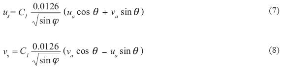
Here, the directions of the coordinate axes are arbitrarily chosen; ua and va are x, y components of the surface wind respectively; C1 is a constant parameter, and the θ angle measures the direction of the resultant drift current vector at the right of the surface wind direction.
A detailed derivation of Eqs. 7 and 8 has been given previously (Adem, 1970) and it is based on the Ekman's formulas. Due to the assumptions from which such equations were derived, the parameter θ and C1 can be arbitrarily chosen from the following range:
45° ≤ q ≤ 90°
0.235 ≤ C1 ≤ 1
Eqs. 7 and 8 are applied considering the surface wind associated to CAO, assuming θ ≤ 90° and C1= 0.235, which corresponds to a resultant drift ocean current where the mixed layer depth is equal to the frictional layer depth. The corresponding normal values for the VS components are computed using the climatic data of surface wind in October, from NOAA–CIRES (Web site: http://www.cdc.noaa.gov).
The second equation of the model represents a balance between mechanical energy and thermal energy in the mixed layer, where the entrainment of colder water is determined according to Kraus and Turner's theory (1967):

In Eq. (9) (detailed in Mendoza et al., 2005), G is the input turbulent kinetic energy from the wind, D is the corresponding dissipation within the layer, and Π(βh) is the solar penetration function, where "one" is considered for complete penetration whereas "zero" for complete absorption. The entrainment of cold water from the thermocline (left hand side term in Eq. 9), takes place due to: an increase in the difference between the generation and dissipation of turbulent kinetic energy induced by surface wind (first term on the right hand side); as well as for a decrease in the buoyancy by cooling at the sea surface (second and third term on the right hand side) due to an increase in sensible and latent heat fluxes. The penetration is reduced when the buoyancy is increased by heating of the mixed layer. On the other hand, such penetration stops (Λ = 0) when the heating surpasses the difference between generation and dissipation of turbulent kinetic energy.
3. The integration method
Eqs. 1 and 9 are integrated into a regular grid of 25 km of resolution on the marine surface of GoM, northwest Caribbean Sea and Atlantic Ocean region close to Florida Peninsula (Fig. 1). The time integration of Eq. (1) is explicit (Euler's method) and regarding Eq. (9) an implicit scheme of backward time finite differences is applied (Mendoza et al., 2005); the time–step used is 15 minutes and centered differences are taken for the spatial derivatives in Eq. (1).

At the first time–step, TS is computed with Eq. (1), assuming that the entrainment is equal to zero and using initial conditions for SST and MLD. Taking this TS, h can be computed with Λ = 1 in Eq. (9), through the successive approximation method of Newton (Carnahan et al., 1969). If in Eq. (3) the first condition is satisfied, then TS and h are obtained for the first time–step, however if the second condition is the one satisfied then h must be calculated taking Λ = 0 in Eq. (9).
As per the second time–step, TS and h computed in the first time–step are taken as initial condition, and the process continues until the required interval time is completed.
The horizontal transport of heat by ocean currents and by turbulent eddies is taken as zero in points of closed boundaries (coasts). In points of open boundaries (in the Caribbean Sea and the Atlantic Ocean region close to Florida), it is assumed that the horizontal transport of heat by turbulent eddies is negligible in comparison with the horizontal transport of heat by ocean currents (–VST• TS), which is computed using observed values for the surface ocean currents and the sea surface temperatures.
4. The cold–air outbreak (CAO)
From the images of geo–potential height and sea level pressure (SLP) obtained from NARR/NCEP, the studied CAO, whose maximum winds took place on Western GoM during October 22–23,1999, had its origin in a high pressure system on the North Pacific Ocean around the Aleutians. Subsequently, it was pushed towards the coasts of Canada and the United States of North America, where it penetrated into the continent between the 18 and 19 October. Such high pressure system, was intensified and pushed towards the south–east, influenced by a jet stream at 200 mb level until to reach the boundary between the United States and México on October 20th. This continental high pressure system (103000Pa) and the low pressure system (101400Pa) on the south–east of the GoM established a strong zonal gradient of pressure, producing northerly winds system up to 57 km/h with gusts up to 70 km/h. Whence the CAO was classified as intense, similar wind velocities were described in the Gulf of Tehuantepec by Transviña and Barton (1997).
The high pressure system over the north boundary of México, the low pressure system over the GoM and the cold front position in October 20 at 12Z are shown in Fig. 2.

5. The input data
The SST, MLD and atmospheric forcing initial values required for the thermodynamic Eq. (1) and for the equation of balance between mechanical and thermal energies in the mixed layer (Eq. 9, Λ = 1), correspond to October 17 at 18Z. However, as SST and MLD data for the initial condition were not available, we took normal values based on October information (Robinson's, 1973) therefore, we used also normal values for the initial atmospheric forcing. The atmospheric forcing associated with CAO was applied 6 hours later and updated every 6 hours during the whole period, meaning October 18 to 23, 1999. The data were: zonal and meridional components of the surface wind, ua and va respectively; surface air temperature Ta; sea level pressure Pa; surface specific humidity qa and fractional low cloud cover ε, which were obtained from the NARR/NCEP reanalysis data with 32 km resolution and interpolated on the grid points of the model (Fig. 1). The air temperature and specific humidity are available at 2 m level, and zonal and meridional wind components are available at 10 m level.
In order to obtain the uncertainty of the data from NARR/NCEP reanalysis, we make a comparison between these data and the measurements of the two buoys indicated in Fig. 1, using the data from the nearest grid point to each buoy (42002 located at 25.17N, 94.42W and 42003 located at 26.03N, 85.88W) and an objective comparison using an index of agreement (IOA). The IOA reflects the exact degree in which a model computes the size and distribution of a variable, regardless of the units. As for this index variation going from 0 to 1, value 1 indicates perfect agreement between the observed and computed values, while value 0 denotes a complete disagreement (Willmott, 1981).
Figure 2 shows that due to the presence of a dry air high pressure system (103000 hPa) over northern México, a strong zonal pressure gradient is established at sea level, which induces intense northerly winds moving towards the Gulf of México.
The vapor pressure ea is incorporated in the heating functions ES, G3 and G2, and it is particularly crucial to compute the latent heat flux, which can be expressed with the well known formula:

Where ra, is the air density at sea level, L is the latent heat of vaporization, Pa is the SLP, Va is the surface wind speed and es (TS) is the saturation vapor pressure at the SST. The coefficients of vertical turbulent transport of latent heat (CE) and sensible heat (CH), depends on stable or unstable case, according to sign of the Richardson number (Huang, 1978), which is expressed in terms of the acceleration of gravity, the square of wind speed, the SLP, the difference between the SST and Ta, and of [0.981eS (TS) – ea].
The vapor pressure in the model is computed with SLP and the specific humidity (qa) at 2 m level from the NARR/NCEP reanalysis of 32 km resolution, using:

In the buoys, the vapor pressure is computed taking data from Ta and relative humidity Ua in the following equation:

Therefore, in the model the importance of the effect of dry air from the CAO is basically determined by the difference [0.981eS (TS) – ea].
Figures 3, 4 and 5 show the surface air temperature, the vapor pressure and the surface wind speed from the NARR/NCEP reanalysis and buoys, respectively.


The wind speed, temperature and humidity (determined by ea) show significant variations at the time the frontal system (CAO) passed over the buoys: on the buoy 42002, on day 19/12Z to 20/18Z, the wind speed (Fig. 5a) increased from ~4 to 16 m s–1, while the surface air temperature (Fig. 3a) decreased 4 °C from ~27 to 23 °C. At the same time, the vapor pressure (Fig. 4a) also experienced a decrease from 34 to 25 mb which continued until day 22/12Z. On buoy 42003, the wind speed (Fig. 5b) increased suddenly a little later, from ~3 to 12 m s–1 during the days 20/18Z to 21/00Z, and then maintained an average speed of ~10 m s–1 during the days 21/00Z to 23/18Z. For its part, the surface air temperature (Fig. 3b) showed a decrease of ~26 to 23.5 °C from the day 21/06Z to 23/06Z, while the vapor pressure (Fig. 4b) fell from ~23 to 21mb. Therefore the arrival of the frontal system to each of the buoys is characterized by a substantial increase in the intensity of the surface wind, and a decrease in the temperature as well as in humidity at the sea surface level.
The vapor pressure values computed with observed data of relative humidity and air temperature were consistently greater than those computed with the NARR/NCEP reanalysis. On the other hand, the corresponding values computed for buoy 42003 (Fig. 4b) were in fact constant throughout the whole period and considerably smaller than the computed values with the NARR/NCEP reanalysis, such difference may be due to some calibration problem in the sensor of humidity in this buoy.
The IOAs shown in Table I, give us a certain degree of confidence in the data from NARR/NCEP reanalysis for use them in the model, except by the vapour pressure computed for the buoy 42003.

6. Analysis of the experiments and results
Buoys 42002 and 42003 also provided values of SST whose changes related to the initial condition (17 October at 18Z) appear in Fig. 6 (dotted line). These changes were compared with the corresponding computed SST changes, for the cases in which the entrainment was either included or not (continuous and dash–dotted lines, respectively in the same figure).
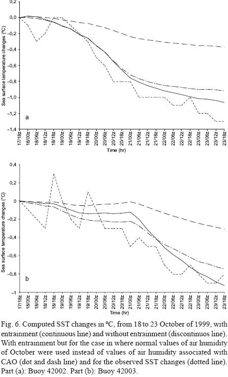
The SST changes were markedly influenced by the wind speed at surface level as it is evident since October 19 at 06Z, when an increment in the wind speed (within a lapse of 30 hours the intensity increased 11m s–1) was registered in buoy 42002. This wind brought as a consequence a decrement in the slope of the curve of the computed SST changes, which coincides with the corresponding changes observed (Fig. 6a). In October 21 at 00Z a suddenly increase in the wind speed appeared in buoy 42003 (within a lapse of 12 hours the intensity increased 8 m s–1) producing a decrement in the slope of the curve of the computed SST changes, in accordance to the corresponding changes observed (Fig. 6b).
At the end of the considered period (October 23 at 18Z) the incorporation of the entrainment term in the thermodynamic equation (Eq. 1), produced a cooling with respect to the non–entrainment case of approximately 0.7 °C near to the buoy 42002 (Fig. 6a) and of 0.6 °C near to buoy 42003 (Fig. 6b). The results show that the incorporation of the entrainment in the model gives a better approach to the observed SST changes, which is also demonstrated by the IOA in the last two columns of Table I.
Fig. 7 shows the computed MLD changes in the region of the two buoys (those with entrainment are presented in continuous line, while those without entrainment as discontinuous line). Here, the influence from the wind speed in the curve of the thermocline's deepening was more important in the first three days since the wind on the buoy 42002 was intensified (dot and dash line) also, in this case a change to minor slope of the curve corresponds to decrement in the intensity of the wind on 20/12Z. In the buoy 42003 the intensification of the wind beginning on day 21/00Z, produced an increase in the slope of the curve. The incorporation of entrainment in the Eq. (1), did not have an important effect on the MLD during the first half of the period, but at the end of the CAO period (October 23, at 18Z) the computed MLD without entrainment was ~9% greater than with entrainment for buoy 42002 and ~15% for buoy 42003.

Figures 8 and 9 show the contributions to the cooling in the mixed layer near to the buoys due to different terms in Eq. (1) (hand right side). In Fig. 8, the most important contribution to the cooling is given by turbulent entrainment of cold water from the thermocline (HWE) followed by the latent heat flux (HG3) and sensible heat flux (HG2). At the time the surface wind was intense the inclusion of air humidity (originated by vapor pressure) in association with CAO, produced a cooling by a latent heat flux (HG3) in the region of both buoys. This cooling was greater than the one based on normal values of air humidity obtained in October (HG3N).


At the end of period, dry air from the CAO substantially increased the cooling of the sea surface due to increase of evaporation. Comparison between the continuous line and the dot and dash line on Fig. 6, shows that this increase is of ~0.15 °C in buoy 42002 and of ~0.20 °C in buoy 42003.
The net radiation produced heat in the mixed layer (HES), associated mainly to solar radiation throughout the period.
The model's low cloud cover (CLDC) established a balance of long wave radiation that prevented the cooling of the oceanic surface; nevertheless, the cloud albedo prevented the entry of solar radiation producing therefore cooling of the surface. The final result was that the effect of cooling by cloud albedo dominated over the greenhouse effect of the clouds; in other words, an increase in the cloud cover produced a decrease in heating by radiation, and conversely, a decrease in the cloud cover produced an increase in heating by radiation.
The greater cooling in buoy 42002 (Fig. 8a) took place during the day 20/12Z, just when the intensity of the wind was at maximum values, whereas in buoy 42003 (Fig. 8b) the greater cooling occurred on day 21/00Z, under the maximum wind intensity values as well.
The greater contribution to cooling of the mixed layer by horizontal transport of thermal energy in buoy 42002 (Fig. 9a), was mainly due to advection of seasonal ocean currents (HADSW) and turbulent eddies (HTU), whereas in buoy 42003 (Fig. 9b) it was due to advection of wind drift (HADEK) and seasonal ocean currents (HADSW). Cooling by horizontal transport of thermal energy was of the same order than the one produced by the sensible heat flux.
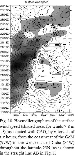
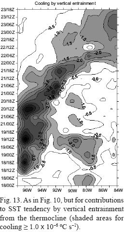
Hovmöller graphics demonstrate the effects of the CAO on the SST tendency (left hand term in Eq. 1) from the west coast of the GoM (97W) to the west coast of Cuba (84W) along 23N (straight line AB in Fig. 1). In Fig. 10 the surface wind speed associated with the CAO (shaded areas for wind ≥ 8 m s–1) shows a displacement towards east and gusts up to 19 m s–1 (70 km h–1) near the west coast of the GoM (from October 20 at 12Z to October 21 at 00Z). The SST tendency is shown in Fig. 11 (shaded areas for cooling ≥ 1.5 × 10⁻⁶ °C s–1). Figures 12 and 13, respectively, show the contributions to the SST tendency in Eq. (1) by thermal forcing in the mixed layer (shaded areas for cooling ≥ 0.5 × 10⁻⁶°C s–1) and by vertical entrainment from the thermocline (shaded areas for cooling ≥ 1.0 × 10⁻⁶ °C s–1). On the other hand, contributions to the SST tendency due to the horizontal transport of thermal energy are shown as follows: in Fig. 14 when the cooling is given by advection of seasonal ocean currents (shaded areas for cooling ≥ 1.5 × 10⁻⁶ °C s–1), in Fig. 15 when it is given by advection of drift ocean currents (shaded areas for cooling ≥ 0.2 × 10⁻⁶ °C s–1) and in Fig. 16 when it is given by advection of horizontal turbulent transport (shaded areas for cooling ≥ 0.3 × 10⁻⁶ °C s–1).


An analysis of Figure 11–16 shows the signal from the wind associated to the CAO, with a clear displacement towards east and reflected in the SST tendency for thermal forcing, for vertical entrainment and also for horizontal advection by the drift ocean currents.
The most important contribution to the entrainment velocity in Eq. (4) shown in Figure 17 (shaded areas for values ≥100 × 10–6 m s–1), was produced by the deepening of the mixed layer as is shown in Fig. 18 (shaded areas for velocities ≥100.0 × 10⁻⁶ m s–1), which reached velocities of ~360 × 10–6 m s–1 in regions where the wind was more intense (~18 m s–1); on these same regions the upwelling by Ekman's pumping shown in Fig. 19 (shaded areas for values ≤10.0 × 10⁻⁶ m s–1) reached values of –60 × 10–6 m s–1.


In relation to the Ekman's pumping velocity, the wind shear stress in the east direction produced a downwelling near to the west coast on day 20/00Z as well as an upwelling, which was spread towards east from longitude ~96 to 87W.
At 00Z on the last day of the period (October 23, 1999), the CAO left on the half western of the GoM a cooling between ~0.8° and 2.0 °C, as well as a deepening of the mixed layer between 30 and 90 m as it is shown in Fig. 20.

7. Concluding remarks
Our results suggest that the entrainment of cold water from the thermocline, whose main component was the deepening of the mixed layer, turns out to be the most determining factor for the cooling, followed by the latent and sensible heat fluxes. However, in this model the cooling in the mixed layer by entrainment, depends essentially on the prescription of temperature located immediately below the thermocline, which was determined from the observed normal values of MLD, SST and sea temperatures at 150 m depth according to the experiments. Nevertheless, our results in the SST changes induced by the atmospheric forcing and associated with the CAO show a good agreement with the corresponding observed values in both buoys, one in the western region and the other in the eastern region of the GoM.
During the CAO period, the sensible and latent heat fluxes produced cooling, whereas the balance of short and long wave radiation produced heating in the sea surface. Such heating was reduced when the cloudy cover was increased. In these regions the humidity changes associated with the CAO, had a significant effect on the latent heat flux and therefore in the cooling of the sea surface.
It is assumed in this model that the ocean current velocity in the mixed layer is a superposition of the normal seasonal ocean current velocity and the drift ocean current velocity, this last as a product of the intensity of the winds associated with CAO. We found that the advection by Ekman's drift ocean currents produces a cooling with the signal of the surface wind speed, whereas the advection by seasonal ocean currents, produces cooling mainly during the whole period of the CAO as could be observed along 23N and from 98 to 84W.
When the CAO finished, almost the half western of the GoM underwent a cooling between 0.8 and 1.5 °C and a thermocline's deepening between ~30 and 90 m. These results suggest that from October to March the winds produced by the cold–air outbreaks may be the main cause of the cooling of the sea surface in the GoM.
Acknowledgements
This work was supported by the "Programa de Apoyo a Proyectos de Investigación e Innovación Tecnológica" of the Universidad Nacional Autónoma de México. Research Project: "PAPIIT: IN108705–2". Thanks to Rodolfo Meza for his valuable commentaries with respect to the meteorology of cold–air outbreaks and to Berta Oda for the computational technical support.
References
Adem J., 1970. On the prediction on mean monthly ocean temperature. Tellus 22, 410–430. [ Links ]
Alexander R. C. and J. W. Kim, 1976. Diagnostic model study of mixed–layer depths in the summer North Pacific. J. Phys. Oceanogr. 6, 293–298. [ Links ]
Alexander M. A., 1992. Midlatitude atmosphere–ocean interaction during El Niño. Part I: The North Pacific Ocean. J. Climate 5, 944–958. [ Links ]
Bleck R., H. P. Hanson, D. Hu and E. B. Kraus, 1989. Mixed layer–thermocline interaction in a three–dimensional isopycnic coordinate model. J. Phys. Oceanogr. 19, 1417–1439. [ Links ]
Busalacchi A. J. and J. J. O'Brien, 1981. Interannual variability of the equatorial Pacific in the 1960's. J. Geophys. Res. 86, 10 901–10 907. [ Links ]
Camp N. T. and R. L. Elsberry, 1978. Oceanic thermal response to strong atmospheric forcing. II. The role of one–dimensional processes. J. Phys. Oceanogr. 8, 215–224. [ Links ]
Carnahan B., H. A. Luther and J. O. Wilkes, 1969. Applied numerical methods, Wiley & Sons, 604 pp. [ Links ]
Kraus E. B. and J. S. Turner, 1967. A one dimensional model of the seasonal thermocline, II. The general theory and its consequences. Tellus 19, 98–106. [ Links ]
Mendoza V. M., E. E. Villanueva and J. Adem, 2005. On the annual cycle of the sea surface temperature and the mixed layer depth in the Gulf of México. Atmósfera 18, 127–148. [ Links ]
Niiler P. P. and E. B. Kraus, 1977. One–dimensional models of the upper ocean. In: Modelling and prediction of the upper layers of the ocean (E. B. Kraus Ed.). Pergamon Press, 143–172. [ Links ]
Nowlin W. D. and C. A. Parker, 1974. Effects of a cold–air outbreak on shelf waters of the Gulf of México. J. Phys. Oceanogr. 4, 467–486. [ Links ]
O'Brien J. J., R.M. Clancy, A. J. Clarke, M. Crepon, R. Elsberry, T. Gammelsrod, M. MacVean, L. P. Röed and J. D. Thompson, 1977. Upwelling in the ocean: two– and three–dimensional models of upper ocean dynamics and variability. Modelling and prediction of the upper layers of the ocean (E. B. Kraus Ed.). Pergamon Press, 178–228. [ Links ]
Price J. F., 1981. Upper ocean response to a hurricane. J. Phys. Oceanogr. 11, 153–175. [ Links ]
Qu T., 2001. Role of ocean dynamics in determining the mean seasonal cycle of the South China Sea surface temperature. J. Geophys. Res. 106, C4, 6943–6955. [ Links ]
Qu T., 2003. Mixed layer heat balance in the western North Pacific. J. Geophys. Res. 108, C7, 3242. doi:1029/2002JC001536. [ Links ]
Robinson M. K., 1973. Atlas of monthly mean sea surface and subsurface temperature and depth of the top of the thermocline Gulf of México and Caribbean Sea. Scripps. Inst. Ocean., Univ. California, San Diego. SIO Ref. 73–8. [ Links ]
Schopf P. S. and M. A. Cane, 1983. On equatorial dynamics, mixed layer physics and sea surface temperature. J. Phys. Oceanogr. 13, 917–935. [ Links ]
Transviña A. and E. D. Barthon, 1997. Los "Nortes" del Golfo de Tehuantepec: la circulación costera inducida por el viento. Contribuciones a la Oceanografía Física en México. Monografía 3, Unión Geofísica Mexicana, 25–46. [ Links ]
Villanueva E. E., V. M. Mendoza and J. Adem, 2006. Effect of an axially–symmetric cyclonic vortex on the sea surface temperature in the Gulf of México. Atmósfera 19, 127–143. [ Links ]
Willmott C. J., 1981. On the validation of models. Phys. Geogr. 2, 184–194. [ Links ]

