A statistical study of seasonal winter rainfall prediction in the Comahue region (Argentina)

 

M. H. GONZÁLEZ
Departamento de Ciencias de la Atmósfera y los Océanos – Facultad de Ciencias Exactas y Naturales, Universidad de Buenos Aires, Buenos Aires, Argentina Centro de Investigaciones del Mar y la Atmósfera – Consejo Nacional de Investigación Científica y Tecnológica, Universidad de Buenos Aires, Buenos Aires, Argentina and Centro de Investigaciones del Mar y la Atmósfera – 2° piso, Pabellón II, Ciudad Universitaria, 1428 Buenos Aires, Argentina, Corresponding author; e–mail: gonzalez@cima.fcen.uba.ar

 

M. M. SKANSI
Servicio Meteorológico Nacional – Argentina

 

F. LOSANO
Autoridad Interjurisdiccional de las Cuencas de los Ríos Limay, Neuquén y Negro – Argentina

 

Received November 12, 2009; Accepted May 7, 2010

 

RESUMEN

El objetivo del presente estudio es establecer las posibles causas que determinan la variabilidad de la precipitación en el período mayo–junio–julio (MJJ) en la cuencas de los ríos Limay y Neuquén. Para establecer la existencia de patrones de circulación previos a este trimestre indicativos de la variabilidad interanual de la precipitación acumulada en MJJ, se correlacionó la precipitación media en el área en cada una de las cuencas con diferentes predictores durante el trimestre precedente (febrero–marzo–abril). Los resultados indicaron que la precipitación en MJJ en ambas cuencas está relacionada con la temperatura de la superficie del mar y las alturas geopotenciales en diferentes niveles observadas previamente en áreas específicas del océano Indico y del Pacífico Sur, tal vez debido a los trenes de onda que se inician en esas zonas y que al llegar a proximidades de la Patagonia se manifiestan como sistemas precipitantes. También se observaron buenas correlaciones con la temperatura de la superficie del mar en el Atlántico, en la costa de Brasil y Argentina asociada al ingreso de vapor hacia el continente y con el viento zonal y meridional en las inmediaciones de la cuenca, responsables de la advección de aire húmedo. La aplicación de esquemas de predicción utilizando una regresión lineal múltiple dio como resultado que las variables elegidas explican el 51% de la variabilidad de la lluvia en MJJ en la cuenca del Limay y el 44% en la del Neuquén. El esquema se validó utilizando la metodología de validación cruzada, obteniendo correlaciones significativas entre la precipitación observada y la pronosticada en ambas cuencas. El análisis de la lluvia del invierno 2009 mostró que los indicadores de gran escala fueron útiles para detectar con anticipación la precipitación del invierno.

 

ABSTRACT

The aim of this study is to detect the possible causes of the May–to–July rainfall (MJJ) over the Limay and Neuquén river basins. In order to establish the existence of previous circulation patterns associated with interannual rainfall variability, the mean areal precipitation in each one of the basins was correlated to some predictors during the previous three month period (February–March–April). The result is that MJJ rainfall in both basins is related to sea surface temperature and geopotential heights at different levels previously observed in some specific areas of Indian and Pacific Oceans, probably due to wave trains which begin in those areas and then displace towards the Argentine Patagonia coast, thus generating precipitation systems. There are also observed significant correlations with sea surface temperature in the Atlantic Ocean over Brazil and the Argentine coast, associated with the water vapor income into the continent and with zonal and meridional wind over the basins, related to humid air advection. The prediction schemes, using multiple linear regressions, showed that the selected variables are the cause of the 51% of the MJJ rainfall variance in the Limay river basin and the 44% in the Neuquén river one. The scheme was validated by using a cross–validation method and significant correlations were detected between observed and forecast rainfall. The 2009 winter rainfall was analyzed and showed that circulation indicators were useful to predict winter rainfall.

Keywords: Seasonal prediction, precipitation, multiple linear regression, sea surface temperature, atmospheric circulation.

 

1. Introduction

The Andes Mountain range lies all along the western part of South America. Its height falls from 3000 to 1500 m south of 38° S, in Argentina, and therefore moist air can enter the continent from the Pacific Ocean. Precipitation amounts decrease significantly towards the east (Atlantic Ocean). The Comahue region is located in the area of the Andes range, between 38° and 43° S. There, the low level flow prevails from the west and rainfall is a typical feature in winter. Two important rivers run in this area: Limay and Neuquén. Most of the energy resources of Argentina come from hydroelectric stations operating in the region, like "El Chocón" and "Piedra del Águila". Obviously, energy production is highly sensitive to water availability and therefore, to the interannual rainfall variability. That is the reason why seasonal rainfall forecast is relevant for planning such activities. The scientific basis of the seasonal climate predictability lies in the fact that slow variations in the earth's boundary conditions (i.e. sea surface temperature or soil wetness) can influence global atmospheric circulation and thus precipitation. As the skill of seasonal numerical prediction models is still limited, it is essential the statistical study of the probable relationships between some local or remote forcing and rainfall. Some authors have analyzed these relationships in the southern hemisphere. Gissila et al. (2004) related sea surface temperatures with Ethiopian rainfall; Reason (2001) did it for South Africa and Zheng and Frederiksen (2006) derived a linear regression model to predict rainfall in Australia. Singhrattna et al. (2005) developed two methods, a linear regression method and a polynomial–based non parametric method for forecasting Thailand summer monsoon rainfall. The last one showed significant skill especially during extreme wet and dry years.

The interannual rainfall variability of the region under study has been partially related to El Niño–Southern Oscillation (ENSO) by many authors. For example, positive correlations between the Southern Oscillation Index (SOI) and precipitation anomalies in the Andes mountains, between 45° S and 55° S, have been found by Schneider and Geis (2004) and rainfall decreased about 15% during strong warm phase of ENSO. Aceituno (1988) and Aceituno and Garreaud (1995) showed that winter precipitation was greater than normal in Central Chile during negative phases of the SOI. Besides, rainfall increased when a greater number of blocking events over the South Pacific were present during warm ENSO events (Rutland and Fuenzalida, 1991; Montecinos and Aceituno, 2003). Compagnucci and Vargas (1998) showed that winters that precede a mature phase of El Niño (La Niña) were characterized by larger (smaller) amounts of snow over the Andes, north of 36° S, which contributed to increase (decrease) the water volume of the rivers. Although ENSO is probably the best comprehended remote forcing, there are some studies which deal with the relationships between rainfall and other circulation patterns. Hence, Compagnucci and Araneo (2005) detected that the interannual variability of river discharges along the Andes was influenced by variations in the Pacific Ocean surface, and that those conditions were not associated with ENSO. Gonzalez and Flores (2008) showed negative correlations between winter rainfall in the Andes mountain range in Central Argentina and sea surface temperature in the tropical Indian Ocean. Gonzalez and Vera (2009) observed the same pattern analyzing interannual rainfall variability in the Comahue region using a principal component analysis. The aim of this paper is to detect the possible relationships between winter rainfall in the Comahue region and both, sea surface temperature in the oceans and atmospheric circulation patterns observed previously to the rainy season.

The paper is organized as follows: Section 2 describes the dataset and the methodology; Section 3 presents the rainfall features in Limay (LRB) and Neuquén (NRB) rivers basins (section 3.1), their association with atmospheric circulation and SST anomaly patterns (3.2) and the building of regression models to estimate winter rainfall in both basins (section 3.3), and Section 4 presents the main conclusions.

 

2. Data and methodology

Monthly rainfall data derived from 34 stations from different sources (Servicio Meteorológico Nacional, Secretaría de Hidrología and the Autoridad Interjurisdiccional of the Limay, Neuquén and Negro rivers basins) were used in this study. The stations are located in the southern Andes region between 37° and 43° S, encompassing the Argentinean provinces of Neuquén (Fig. 1). This province limits with Neuquén river in the north and Limay river in the south. The period under study goes from 1975 to 2007. It was selected because all the stations have less than 20% of missing monthly rainfall data and their quality has been carefully proved. The analysis concentrates on southern winter rainfall.

Monthly sea surface temperatures (SST), 500 hPa (G500), 1000 hPa (G1000) and 200 hPa (G200) geopotential heights, zonal (U) and meridional (V) winds at 850 hPa from National Center of Environmental Prediction (NCEP) reanalysis were also used (Kalnay et al., 1996). Monthly anomalies were determined removing the long–term monthly means from the original values.

Low frequency variability of the precipitation series was analyzed using a linear trend method of minimum squares, and statistics significance was tested using t–Student and Mann Kendall tests (Mann, 1945).

The area of study is limited by two important rivers, the Limay river in the south and the Neuquén river in the north. Although it is a small area, some differences were detected over both basins. Twenty stations –out of the 34 over the area– are located inside the Neuquén (12 stations) and Limay (8 stations) basins and they were used to analyze rainfall behavior in each basin. Therefore, two mean rainfall series were constructed as the average of monthly precipitation of 12 stations in NRB, and eight stations in the LRB, in order to be representative as from the precipitation over each one of the basins (Fig. 1) .

Simultaneous and lagged correlations were calculated to find the existing relation between winter rainfall in the NRB and LRB and SST, G1000, G500, G200, U and V. The results allow to define some predictors, which were used to develop a statistical forecast model using the forward stepwise regression method (Wilks, 1995), which retained only the variables correlated with a 95% significance level. Forward stepwise regression is a model–building technique that finds subsets of predictor variables that most adequately predict responses on a dependent variable by linear regression, given the specified criteria for adequacy of model fit (Darlington, 1990). The basic procedures involve identifying an initial model, repeatedly altering the model at the previous step by adding a predictor variable following a fixed criterion, and terminating the search when stepping is no longer possible as to the criteria. Predictors available to carry out the regression scheme were carefully selected, based on statistical significance and physical reasoning.

 

3. Results and discussion

3.1 General precipitation features

Linear trend approximation is a simple way to evaluate the observed change in a time series (Darlington, 1990; Wilks, 1995) and it represents precipitation time evolution efficiently in a given period. Figure 1 shows annual rainfall linear trends in the area under study, calculated with observed data in 34 stations, registered during the 1975–2007 period. Rainfall decreases less than 12 mm/year all over the region and trends were statistically significant only in a few stations very near the Andes range. This result agrees with Barros and Castañeda (2001) who calculated linear trends using a shorter period.

Mean series in both regions (NRB and LRB), calculated as it was detailed in the previous section, were considered. Mean monthly rainfall evolution for them is depicted in Figure 2. The main feature is a defined annual cycle with a peak in late autumn and winter over both basins. This is the reason why this paper mainly deals with the period from May to July (MJJ), representative of southern winter rainfall. Furthermore, rainfall in LRB exceeds the NRB all along the year.

3.2 Relationship between winter rainfall and sea surface temperature and atmospheric circulation

There are some evidences that rainfall patterns in the study region are related to remote forcing like El Niño–Southern Oscillation (ENSO) phenomenon (Compagnucci and Vargas, 1998; Grimm et al., 2000) but there must be considered the presence of other remote forcing (Reason, 2001; Gissila, 2004; Singhrattna et al., 2005; Zheng and Frederiksen, 2006). It is important to notice that remote forcing can increase the chances of success of seasonal predictability because it can be extended out to longer ranges based on the influences of slowly evolving boundary conditions on the atmospheric circulation, such as the sea surface temperature or the soil wetness and, hence, seasonal climate can tilt in a specific direction.

The previous circulation anomalies associated with MJJ precipitation over LRB and NRB are explored in order to identify the key elements of the atmospheric circulation that promote or inhibit rainfall anomalies in the study region. Correlation maps between the MJJ rainfall series, spatially averaged in each one of the basins (LRB and NRB), and the February to April (FMA) seasonal anomalies of SST, G1000, G500 and G200, were made to describe the patterns of circulation which were present before the winter rainfall and as a consequence, some predictors be defined. The 1975–2007 data period was used. During 33 years, the correlation required for significance at the 95% level is 0.35. The areas with high correlation were used to define some predictors. Predictors to carry out the regression scheme will be carefully selected, based on statistical significance and physical reasoning. Similar maps were also made for U and V, indicative of the low–level flow across the Andes, responsible of the entrance of humid air into the region.

First, the results derived from LRB will be detailed. A lagged correlation map between MJJ rainfall in LRB and FMA SST is displayed in Figure 3. Negative correlation values along the tropical band in the Indian Ocean (7–20° S; 80–120° E) were observed and a predictor I1 could be defined. To make it clearer, Table I shows the predictors that will be described in this section. The areas with significant correlation persist when simultaneous correlation is performed (figure not shown). Some other authors have pointed out relationships between rainfall and SST in the Indian Ocean. Zheng and Frederiksen (2006) showed that SST conditions in central Indian Ocean in the period March–May are related to winter rainfall variability in New Zealand; Reason (2001) and Gissila (2004) described links between Indian Ocean SST variability and rainfall in South Africa and Ethiopia, respectively. In South America, González and Vera (2009) found significant correlations between the first leading rainfall pattern, positioned near LRB and Indian SST. Some other areas with significant correlation were detected and are shown in Figure 3. One of them was positioned in 0–10° S; 110–85° W (P1) and it is associated with the El Niño–Southern Oscillation (ENSO) phenomenon, indicating that rainfall is mainly related to the cold phase of ENSO. Two areas in mid–latitudes, one positioned in the western South Pacific (30–40° S; 180–160° W) (P2), and the other in the eastern South Pacific (35–45° S; 110–90° W) (P3) appear to have influence on South American rainfall through Rossby wave propagation (Kalnay et al., 1986; Mo 2000), as explained in the next paragraph. Negative correlations were found in the Atlantic Ocean (5–25° S; 40–20° W) (A1) in tropical Atlantic and in 45–50° S; 55–35° W (A2) in mid–latitudes, which are related to the entrance of humid air into the continent through the Atlantic height.

The correlation maps between G500 (Fig. 4), G1000 and G200 (figures not shown) anomalies for FMA and MJJ rainfall in LRB, show a well–defined wave train extended from the Indian Ocean towards South America with large amplitudes in the Pacific South America sector. This wavelike pattern is also obvious for the simultaneous correlations (not shown). This pattern resembles the third leading pattern of circulation detected by Mo (2000) when she describes 500 hPa geopotential height interannual variability (Pacific South American Pattern, PSAP) which is characterized by a wave train emanating from the tropical western Pacific towards the south. She also describes linkages between circulation regime and SST and the PSAP association with the tropical Indian Ocean SST anomalies on quasi–biennial timescales. Therefore, the correlation between SST and MJJ LRB (Fig. 3) also shows anomalies in the Indian Ocean, which are consistent with those related to PSAP, described by Mo (2000). Other authors have also found the quasi–biennial signal in SST near Australia (Trenberth, 1975) and over the Indian Ocean (Allan et al., 1995); they related it to the development of the Asian monsoon, which reaches its maximum in the period September–November and proved that only the Indian Ocean anomalies remained significant in other seasons. Another important feature in Figure 4 is the anticyclonic anomaly positioned over central Argentina and the western coast of the Pacific Ocean, which is part of the wave train pattern described below. Thus, both the anomalies in the Indian Ocean and the wavelike pattern over the Pacific Ocean are related to the displacement of precipitation systems which arrive to the South American coast and which can go through the southern portion of the Andes mountains (south of 38° S), because these are lower than in the north. Gonzalez and Vera (2009) showed the same wave outline for the first leading winter rainfall pattern. Some predictors were defined in G500 field (Fig. 4): G1 (40–60° S;115–135° E) in Western Pacific in mid–latitudes, G2 (15–30° S; 150–195° E) in Tropical Central Pacific, G3 (5–20° S; 240–280° E) in Eastern Tropical Pacific and G4 (45–55° S; 220–260° E) in Eastern Pacific in mid–latitudes and two more, slightly displaced in the G1000 field, which were called G´1 y G´2 (see Table I).

The correlation map between MJJ rainfall in LRB and U anomalies for FMA (Fig. 5) indicates that precipitation is related to weaken westerly winds south 50°S in the Eastern Pacific and enhanced westerly winds over the continent in the southern portion of Argentina. In fact, this regional pattern is a consequence of the hemispherical behavior, described in the paragraph above and thus, this feature is consistent with the wavelike pattern described in Figure 4. Both the cyclonic anomaly in south–eastern Pacific and the anticyclonic one over central Argentina determine a region of enhanced westerly winds in southern Argentina north 50° S and weaken westerly winds in the Pacific Ocean, southwestern of Argentina. The enhancement of westerly winds in the southern part of the continent and the presence of mountains with a north–south orientation induce an increase of cyclonic vorticity leeward of the Andes, which favours the enhancement of rainy systems. One more predictor was defined as mean U in the area 55–70° S; 130–90° W (Z1). The correlation field with V (Fig. 6) shows two areas with significant correlation, one in 5–15° S; 110–90° W (M1), indicating that rainfall can be associated with enhanced trade winds (cold phase of ENSO), and the other in the South Pacific (40–60° S; 90–80° W) (M2). The first one (M1) described in Figure 3, is consistent with the negative correlation between MJJ rainfall and SST (defined as P1). It shows a tendency towards the rainiest season when La Niña event is present. The second meridional wind predictor (M2) is associated with the anticyclonic anomaly in G500 (Fig. 4) over Argentina. This geopotential height anomaly establishes northerly anomalies over the area where M2 was defined and southerly anomalies over the basin which results less significant than the northerly ones.

The same methodology was applied to MJJ precipitation in NRB. Correlation maps between rainfall in this basin and SST (Fig. 7), G500, U and V (figures not shown) anomalies for FMA show some equivalence and some differences from results obtained for LRB. Figure 7 shows that the area of significant correlation along the Tropical Indian Ocean (I1) in LRB, is not so important in the NRB case and it is restricted to the eastern part of the Indian Ocean. However, an area in the Subtropical Indian Ocean (35–50° S; 95–120° E) (In) shows significant correlation. Moreover, positive correlations are observed in the Subtropical Atlantic Ocean (30–40° S; 35–15° W) (An). The correlation maps with G500, G1000 and G200 show the same wavelike pattern that was detected for LRB (figures not shown). Rainfall in NRB is also enhanced by strong westerly winds (Z1) in the southern part of the continent and when the cold phase of ENSO (M1) is present. These results agree with the ones that have been detected for LRB. A new predictor (Zn) was defined as the mean U in the area (40–50° S; 75–45° W).

3.3 Linear forecast model

To select the best predictors to be used in the multiple linear regression methodology, the correlations between all the predictors defined and NRB and LRB rainfall were calculated (Table II). The choice of input variables for the regression model was done among the predictors described in Table II. Only those with correlation greater than 0.35 were considered because it turned to be significant at a 95% confidence level. However, as the predictors must be independent among each other, some of them were disregarded.

Finally, the input predictors for MJJ rainfall in LRB were I1, P2, P3, A2, G4, G`2, Z1 and M1. The selected model was a forward stepwise regression, which retained only the variables, correlated with 95% significance level. The derived model was:

P = –1724 I1 + 1892 M1 + 51836

where P is the value predicted for the accumulated MJJ rainfall in LRB (in mm x 10). The percentage of variance explained by the model was 54% with a lineal regression coefficient of 0.73. A commonly used measure of strength of the regression is the F–ratio, defined as the relationship between the mean square regression and the mean square error (Wilks, 1995). It is worthwhile that the F–ratio was high because a strong relationship between P and the predictors will produce large mean square regression and small mean square error. As the residual of the regression is independent and follow a normal distribution, under the null hypothesis of no lineal regression, the F–ratio was 17.7 with a p–value of 0.00001, and therefore, the regression model provides reasonably forecast with 95% of confidence. The model can show the importance of the SST in the Tropical Indian Ocean (I1) and the ENSO phase (M1) as good indicators of interannual winter rainfall variability in LRB.

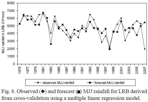
A common approach to better estimate predicting skill is a cross–validation (Wilks, 1995), where n–1 years were used for calibration and the remaining year was used to validate the model. This process was repeated several times with a different year as the validation target in each case. This method is generally strong in the presence of long–term climate variability and is used specially, when the number of data is not so large. In the LRB case the method took 32 years in each calibration and 8 predictors, so there was no possibility of over fitting. In the process of cross–validation, the exclusion of a single year from the data did not cause important changes in the model, and therefore there was no evidence of numerical instability. The observed and forecast MJJ rainfall for LRB is shown in Figure 8. The correlation between them was 0.65 which was significant at 95% confidence level.

The process was repeated for MJJ rainfall in NRB. The input predictors to the multiple linear regression method were: In, An, G`1, Zn and M1. The final model, after applying the forward stepwise methodology, which retained only the variables correlated with 95% significance level, was:

P = –1391 In – 312 G`1 + 23946

where, P is the estimated MJJ rainfall in NRB (in mm x 10). The model explained the 43% of the precipitation variance and the F–ratio was 11.5 with p–value of 0.0002. SST in the Indian Ocean (In) seems to be an important key for rainfall prediction in this basin, too. Furthermore, geopotential heights at low levels in the Pacific Ocean, associated with Rossby wave trains, were a good indicator of rainfall variability (G´1). Figure 9 shows the MJJ observed and estimated rainfall in NRB after applying a cross–validation method. Correlation between estimated and observed rainfall was 0.48.

The skill of the forecast was measured in semi–quantitative terms as follows: the observed and forecast rainfall distribution was categorized in terciles and they were compared by constructing a contingency table (Table III and IV). These contingency tables differ significantly from a random one, using a chi–square test. The "upper" interval refers to values greater than the second tercile, "lower" refers to values less than first tercile, and "normal" to values greater than first and lower than second terciles.

The events "dry" and "wet" were calculated collapsing the 3 x 3 contingency table into two 2 x 2 tables. Each one is constructed by considering the "forecast event" (dry or wet) as opposed to the complementary "non forecast event" (non–dry or non–wet). Some measures of accuracy (Wilks, 1995) were calculated for wet and dry cases in both basins (Table V). The hit rate (H) or the right proportion is the fraction of all the cases when the categorical forecast correctly anticipated the subsequent event. The probability of detection (POD) is defined as the fraction of those occasions when the forecasted event occurred on which it was also forecast. The false alarm relation (FAR) is the proportion of forecast events that fail to happen. The Heidke score (HS) is a relative accurate measure that compares the skill of the forecast with the hit rate that would be achieved by random forecast. The perfect forecast receives Heidke score of one, forecasts equivalent to reference forecast (random) receive score zero. The values in Table V indicate that the efficiency of the method is better in LRB than in NRB and the events "wet" are better detected than the "dry" ones in both basins.

3.4 A case of study

To illustrate the efficiency of this method, the case of MJJ 2009 will be detailed in this section. Figure 10 shows the SST field average in FMA 2009. The anomalies are very weak over the areas where the predictors have been defined in the Indian and Pacific Ocean (I1, P2 and P3), meanwhile there are great positive anomalies in the area where An is defined, indicating the possibility of MJJ rainfall above normal especially in NRB.

The G500 field in FMA 2009 (Fig. 11) shows a wave like pattern with an important negative anomaly in the southeastern Pacific, south of 50° S and a center of positive anomaly over the continent in central Argentina. This regional pattern agrees with the correlation maps detailed for LRB and NRB (Fig. 4), and therefore they are indicative of MJJ rainfall above normal in both basins.

The U pattern in FMA 2009 (Fig. 12) is dominated by positive anomalies (enhanced westerly flow) in the southeastern Pacific Ocean and south of Argentina and weakened westerly winds south 50° S. This pattern reflects a probability of rainfall above normal in LRB and NRB, when compared with Figure 5.

The V field in FMA 2009 (Fig. 13) shows no signal in the area where M1 is defined (ENSO signal) but southern wind is observed over both basins, in accordance with Figure 6. Therefore, this factor collaborates to increase MJJ rainfall in the study area.

Although the predictors selected by the multiple linear regression technique to build the models had really poor signal in FMA 2009, it was possible to analyze the anomaly fields of the different atmospheric variables to propose that MJJ rainfall would be above normal. Figure 14 shows the MJJ 2009 anomalies in Argentina, with data from the Servicio Meteorológico Nacional. The area under study was really dominated by positive anomalies, greater in LRB than in NRB. These anomalies agree with the results obtained when the SST and atmospheric variables anomaly field were analyzed for 2009.

If the derived models were used to forecast MJJ rainfall, the results would be as follows: the LRB model forecasted 512 mm, a value very similar to the upper limit of the normal interval (418 mm, 558 mm). The NRB model forecasted 303 mm when the normal interval is 235 mm, 312 mm. Thus, the method classified the MJJ 2009 as a normal year in both basins.

3.5 The importance of seasonal forecast in dams

LRB occupies an area of 23 600 km² and its mean flow is 734 m³/s. The hydroelectric dams of Alicura, Piedra del Águila, Pichi Picun Leufu and El Chocón are on this river. The hydropower system is approximately 5000 Mw with an annual energy generation of 14 500 Gwh, 20% of the Argentinian budget. The Autoridad Interjurisdiccional de Cuencas (AIC) [Government Bureau of the Limay, Neuquén and Negro river basins] runs the fiscal control of power generation concessionaries, water schedule release and it also controls the management of water use down dams, probability of flooding and high drainage level from irrigated valleys. This structure pretends to rationalize and harmonize water use. A hydrological integrated system is efficient to evaluate the basin water resources in real time including the operative restrictions previously assumed pursuant to legal provisions. A conceptual hydrological model, which uses soil moisture, lake levels, snow melting, and runoff algorithms, generates short and medium term forecasts to determinate flood peaks and runoff volume. Due to the presence of different factors regarding dam management (AIC, power generation concessionaries, electricity distribution concerns), it is necessary to follow certain operating rules as to keep a certain water level of the reservoir. When operating the dam, there are several aspects to be taken into account regarding water level: emergency, flood smoothing, normal and extraordinary levels. This conventional work operation level is not enough because the prospective demand of water depends not only on the meteorological situation but, also on daily electricity demand. Therefore, it is necessary a better understanding of rainfall behaviour over the basin through the knowledge of those predictors, which allows to anticipate seasonal precipitation and the building of statistical models.

The operating levels in Piedra del Águila in 2008, 2009 and 2010 hydrological periods, were set above maximum levels in normal operational management standards. This used to render and still renders an operational and economic benefit from the point of view of hydropower production, because the reservoir operates with higher power, but at the same time, it increases the vulnerability of residents downstream the dam, in case of a major hazard, for example. The system of reservoirs in Limay river has a final capacity of evacuation through the last of its compensating reservoirs located downstream of El Chocón, of 3800 m³/s, a probable maximum flood of 18 000 m³/s and a volume of 12 000 hm³ in 30 days. The discharge capacity of Piedra del Águila is 10 000 m³/s with a maximum volume available for attenuation of 4660 hm³. Thus, it is important to determinate the degree of anticipation and the efficiency of the forecast, in order that the hydrological operator has enough time to restore dam levels which ensure the security of the dam and the residents located downstream.

The correlation results and the statistical model derived in previous section are tools to improve those forecasts. The predictors can be obtained from the data library of the International Research Institute for Climate and Society (IRI, Columbia University, cpt@iri.columbia.edu). This site offers the possibility to get data averaged in time and in a defined region. Moreover, the Climate Predictability Tool (CPT), developed by IRI provides a software package for constructing a seasonal climate forecast model, producing forecasts by taking updated data from NCEP reanalysis. CPT can be used to determine the spatial variability of rainfall in the Comahue region. The technique requires the entrance of FMA predictors previously defined and MJJ rainfall data in some stations of the area for 1975–2007 period. The methodology performs a CCA analysis for both FMA predictor and MJJ rainfall, and correlates them, generating a relation between them. Therefore, CPT allows to forecast rainfall for each individual station in a particular year out of the training period (1975–2007). Finally, a forecast rainfall field was built for that particular year. The predictors considered to apply CCA methodology are those derived from the correlation analysis detailed in previous sections using NCEP reanalysis data (Kalnay et al., 1996).

 

4. Conclusions

The analysis of the mean seasonal cycle of the area under study shows that most of the rain occurs during winter. Negative trends less than 12 mm/year are observed all over the region, but statistically significant only in a few stations very near the Andes mountain range. In order to identify circulation signals related to rainfall interannual variability, two mean areal series (LRB and NRB) were defined as the average of rainfall in some station located in the Limay and Neuquen river basins. To identify predictors, LRB and NRB rainfall was correlated with sea surface temperature, geopotential height and low–level winds observed three months before, which can be used in a regression model. A forward stepwise methodology was used to develop a prediction model and a cross–validation scheme was applied to the period 1975–2007. The analysis for LRB shows that the most important source of predictability comes from the interannual variability of SST in the Tropical Indian Ocean and the ENSO phase. The final prediction model for LRB explained 54% of the rainfall variance and a correlation of 0.65 was calculated between observed and forecast series. In NRB case, SST in the Indian Ocean was an important key for rainfall prediction, but geopotential heights at low levels in the Pacific Ocean, associated with the Rossby wave train that extend along the South Pacific, resulted a good indicator of rainfall variability. The final model for NRB explained 43% of rainfall variance and the correlation between forecast and observed series was 0.48. Correlations with low level flow indicate that precipitation in both basins is related to weaken westerly winds south 50 °S in the Eastern Pacific, enhanced westerly winds over the continent in the southern portion of Argentina, and to enhanced southern winds over the basins. The case of winter 2009 was analyzed and although the predictors selected by the models had no significant anomalies this year, the correlation maps helped to detect the possibility of "normal" to "above normal" rainfall with FMA data.

The fact that changes in the conditions of Pacific and Indian oceans and geopotential heights at different levels were related to interannual winter rainfall variability in this area provides some scope for seasonal prediction in the region. These results are important to operate dams in the Comahue region because the statistical model may be useful to improve the forecast required. This paper intends to contribute to a better knowledge of climate variability, in order to make better seasonal predictions.

 

Acknowledgements

Rainfall data were provided by the Servicio Meteorológico Nacional, the Secretaría de Hidrología of Argentina and the territory authority of the Limay, Neuquén and Negro rivers basins. Images from Figs. 3 to 7 and 10 to 13 were provided by the NOAA/ESRL Physical Sciences Division, Boulder Colorado from their web site: http://www.cdc.noaa.gov. This research was supported by UBACyT X444, UBACyT X160 and CONICET PIP 112–200801–00195.

 

References

Aceituno P., 1988. On the functioning of the Southern Oscillation in the South American sector. Part I: surface climate. Mon. Wea. Rev. 116, 505–524.        [ Links ]

Aceituno P. and R. Garreaud, 1995. Impactos de los fenómenos El Niño y La Niña sobre regímenes fluviométricos andinos. Rev. Soc. Chil. Ing. Hidr. 10, 33–43.        [ Links ]

Allan R. J., J. A. Lindesay and C. J. Reason, 1995. Multidecadal variability in the climate system over the Indian Ocean region during the Austral Summer. J. Climate 8, 1853–1873.        [ Links ]

Barros V. R. and M. E. Castañeda, 2001. Tendencias de la precipitación en el oeste de Argentina. Meteorologica 26, 5–24.         [ Links ]

Compagnucci R. and W. Vargas, 1998. Inter–annual variability of the Cuyo river streamflow in the Argentinean andean mountains and ENSO events. Int. J. Climatol. 18, 1593–1609.        [ Links ]

Compagnucci R. and D. Araneo, 2005. Identificación de áreas de homogeneidad estadística para los caudales de los ríos andinos argentinos y su relación con la circulación atmosférica y la temperatura superficial del mar. Meteorologica 30, 41–54.        [ Links ]

Darlington R. B., 1990. Regression and linear models. McGraw–Hill. New York, 542 pp.        [ Links ]

Gissila T., E. Black, D. I. F. Grime and J. M. Slingo, 2004. Seasonal forecasting of the Ethiopian summer rains. Int. J. Climatol. 24, 1345–1358.        [ Links ]

González M. H. and O. K. Flores, 2008. La posible incidencia de los océanos en la precipitación en los Andes Centrales de Argentina. Memorias del II Congreso Internacional sobre Gestión y Tratamiento Integral del Agua, 5 al 7 de noviembre de 2008, Córdoba, Argentina, 188–197.        [ Links ]

González, M. H. and Vera, C. S., 2010. On the interannual winter rainfall variability in Southern Andes. Int. J. Climatol. 30, 643–657. DOI: 10.1002/joc.1910.        [ Links ]

Grimm A., V. Barros and M. Doyle, 2000. Climate variability in Southern South America associated with El Niño and La Niña events. J. Climate 13, 35–58.        [ Links ]

Kalnay E., K. C. Mo and J. Paegle, 1986. Large–amplitude, short scale stationary Rossby waves in the southern hemisphere: observations and mechanistics experiments on determine their origin. J. Atmos. Sci. 3, 252–275.        [ Links ]

Kalnay E., M. Kanamitsu, R. Kistler, W. Collins, D. Deaven, L. Gandin, M. Iredell, S. Saha, G. White, J. Woollen, I. Zhu, M. Chelliah, W. Ebisuzaki, W. Higgings, J. Janowiak, K. C. Mo, C. Ropelewski, J. Wang, A. Leetmaa, R. Reynolds, R. Jenne and D. Joseph, 1996. The NCEP/NCAR Reanalysis 40 years–project. B. Amer. Meteorol. Soc. 77, 437–471.        [ Links ]

Mann H. B., 1945. Non–parametric tests against trend. Econometrica 13, 245–259.        [ Links ]

Mo K., 2000. Relationships between low frequency variability in the Southern Hemisphere and sea surface temperature anomalies. J. Climate 13, 3599–3610.        [ Links ]

Montecinos A. and P. Aceituno, 2003. Seasonality of the ENSO related rainfall variability in Central Chile and associated circulation anomalies. J. Climate 16, 281–296.        [ Links ]

Reason C., 2001. Subtropical Indian ocean SST dipole events and Southern Africa rainfall. Geophys. Res. Lett. 28, 2225–2227.        [ Links ]

Rutland J. and H. Fuenzalida, 1991. Synoptic aspects of the central Chile rainfall variability associated with the Southern Oscillation. Int. J. Climatol. 11, 63–76.        [ Links ]

Schneider C. and D. Gies, 2004. Effects of El Niño–southern oscillation on southernmost South America precipitation at 53 °S revealed from NCEP–NCAR reanalysis and weather station data. Int. J. Climatol. 24, 1057–1076.        [ Links ]

Singhrattna N., B. Rajagopalan, M. Clark and K. K. Kumar, 2005. Seasonal forecasting of Thailand summer monsoon rainfall. Int. J. Climatol. 25, 649–664.        [ Links ]

Trenberth K. E. 1975. A quassi biennial standing wave in the Southern Hemisphere and interrelations with sea surface temperatures. Quart. J. Roy. Meteor. Soc. 101, 55–74.        [ Links ]

Wilks D. S., 1995. Statistical methods in the atmospheric sciences. An introduction. International Geophysics Series. Academic Press, San Diego, California, USA, 467 pp.        [ Links ]

Zheng X. and C. Frederiksen, 2006. A study of predictable patterns for seasonal forecasting of New Zealand rainfall. J. Climate 19, 3320–3333.        [ Links ]