


Servicios Personalizados
Revista
Articulo
 Inglés (pdf)
 Artículo en XML
 Referencias del artículo
 Enviar artículo por email
Indicadores
-
 Citado por SciELO
 -
 Accesos
Links relacionados
-
 Similares en
SciELO
Similares en
SciELO
Compartir

 Permalink
Atmósfera
versión impresa ISSN 0187-6236
Atmósfera vol.23 no.2 Ciudad de México abr. 2010
The singular role of the atmospheric stability in forest fires
S. DOMÍNGUEZ MARTÍN and E. L. GARCÍA DÍEZ
Facultad de Ciencias Agrarias y Ambientales, Área de Tecnologías del Medio Ambiente, Universidad de Salamanca 37007–Salamanca. Corresponding author: E. L. García Díez; e–mail: elga@usal.es
Received January 14, 2009; Accepted November 26, 2009
RESUMEN
La baja estabilidad favorece un transporte hacia arriba del aire caliente generado en la combustión. Contrariamente, la fuerte estabilidad disminuye la posibilidad de este movimiento vertical. Por lo tanto, las condiciones de baja estabilidad favorecen el desarrollo del fuego. Pero este estudio muestra que la baja estabilidad aumenta la actividad de fuego sólo en condiciones atmosféricas de sequedad. Un análisis estadístico de 70,000 incendios en el período 1993–2005 (julio–septiembre) en Galicia (NW de España) indica que el número diario de incendios es mayor en los días secos con baja estabilidad. Esta dependencia de la estabilidad se invierte en los días húmedos. Los valores más bajos del número de incendios forestales tienen lugar en aquellos días con una baja estabilidad acoplada a una alta humedad. Esta dependencia opuesta de la ocurrencia de fuego respecto a la estabilidad atmosférica provoca resultados muy ambiguos en una correlación simple entre la estabilidad y el número de incendios. Además, este papel opuesto de la estabilidad atmosférica implica también valores ambiguos de los índices de riesgo de fuego que aplican una simple adición de la estabilidad y de la humedad.
ABSTRACT
Low stability favors the upward transport of the hot air generated by combustion. On the contrary, strong stability diminishes the potential for this vertical movement. Therefore, it could be concluded that low stability favors fire development. But this study shows that low stability increases fire activity only in dry atmospheric conditions. Statistical analysis of more than 70,000 fires in the period 1993–2005 (July– September) for Galicia (NW Spain) indicates that the daily number of forest fires is greater on dry days with low stability. This dependence on stability, however, reverses for moist days. The lowest values of the daily number of forest fires occur on those days with low stability coupled with high humidity. This bimodal and seemingly contradictory dependence of fire occurrence with respect to atmospheric stability causes misleading results in simple statistical correlations between stability and the number of fires. Furthermore, this contradictory role of the atmospheric stability implies ambiguous values in risk indices that apply simple numerical addition to stability and humidity.
Keywords: Atmospheric stability, moisture, Haines Index, GD index, Galicia, Spain.
1. Introduction
Meteorological parameters are clearly a critical factor influencing the occurrence, behavior and development of wildland fires (Flannigan and Harrington, 1988). Fire is inherently a matter of vertical fuid dynamics and, consequently, he vertical structure of the atmosphere must play an important role in fire development. Crosby (1949), Taylor et al. (1971, 1973), Reifsnyder (1977) and others clearly established the association of atmospheric instability with firegrowth and development.Later, Haines (1988) and García Díez et al. (1994a) presented indices (here noted as the HI and the GD indices, respectively) which include stability of a near–ground atmospheric layer coupled to humidity at the base of this layer. Chunmei et al. (2003) include stability for several laboratory experiments. Others, such as Potter et al. (2003) and Jenkins (2004), include stability in terms of convective available potential energy (CAPE), convective inhibition (CIN) and other conventional parameters from atmospheric thermodynamics. At present, atmospheric stability is accepted as an important regulator for fire but other studies asses it differently (Mc Arthur, 1996).
However, many scientists and managers have pointed out the influence of multiple weather variables, including stability, with the concept of a fire index (Haines, 1988; García Díez et al., 1994a; Mc Arthur, 1996). Over the years and in different countries “risk” is sometimes referred to as “potential,” “danger,” or “hazard.” In this paper we have used “risk”. While it is theoretically possible to use multiple variables directly to assess fire risk, weighing the variables is too complex for operational application. A suitable index of risk of fire must have several specific properties. First, it must have a clear correspondence with the likelihood or severity of fire activity. Second, the index must be consistent with scientific methods, theories and parameters. Third, a risk index must be unambiguous, thus, the input variable combinations that yield a particular index value must correspond to comparable levels of fire activity. Failure to take these three properties into account could cause false alarm or under prediction, and the purpose of a suitable index must be exactly to detect the risk of fire.
This study examines atmospheric stability, atmospheric moisture, and their use in fire risk indices. The suitable relationship between fire activity and atmospheric stability in fire risk indices will be discerned.
2. Methods
In this paper we have used the GD and Haines indices. García Díez et al. (1994a, 1994b, 1996b) developed the former index, which differentiates four types of day according to values of atmospheric stability (e) and humidity, more precisely saturation deficit, (D). These values classify the day in four types as shown in Figure 1.
The stability parameter in the GD model is defined as:
e = S700–S850
in which S is the Montgomery Potential (Arakawa and Schubert, 1974):
S = CpT + gz
where Cp is the specific heat of dry air at constant pressure (1004 J kg–1 °K–1); T the absolute temperature (Kelvin degrees, 273 Kelvin degrees is equal to ° Celsius degree in SI), g acceleration due to gravity (9.8 m s–2) and z geopotential height (meters).
The subscripts 700 and 850 indicate the pressure levels (hectopascal) in which S is determined. High values of e indicate a stable air mass.
The saturation deficit (D) is given by:
D = L (q*–q)850,
where L, is the latent heat of vaporization (2.5x10⁶ J kg–1) and q* and q the saturated specific humidity and specific humidity, respectively (both expressed in kg of water substance per kg of air). The subscript 850 indicates that these values in the 850 hPa level are measured. High values of D indicate a dry air mass.
At 0000 UTC (Universal Time Coordinated), e and D, according to conventional radiosonde data, can be evaluated. Thus, after 0000 UTC, the type of day can be easily known (Fig. 1). Alternatively, since e and D can be provided by numerical weather forecasts, the type of day in standard forecast can be determined, as well.
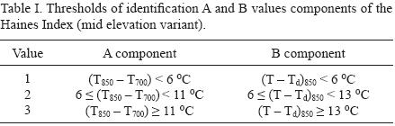
The Haines (1988) Index (HI) , has three variants according to surface elevation over the sea. For this study, the mid–elevation variant is most appropriate. All variants of the HI include a stability component (A) and a moisture component (B). For the mid–elevation variant, the A component is obtained by temperature difference between 850 and 700 hPa, and the B component by dew point depression in 850 hPa, both at 0000 UTC. These differences of temperature are linked with values (1, 2 or 3) of A and B, according to a threshold value (Table I). The results of A and B are added to yield a final value of the HI, located between 2 and 6. Numeric values of 2 and 3 are considered very low risk of large–erratic wild land fire, 4 indicates low risk, 5 is moderate risk, and 6 is high risk.
In this study a brief comment about application of the HI is required. Initially, the Haines Index was designed by its author for fires over 400 hectares under low wind conditions (plume dominated fires). Generally, these criteria are not met in the fires considered in this work, since we have considered all kinds of fires. Therefore, the results will not be directly evaluated for such conditions.
Note that any mathematical addition (stability plus humidity) is not involved by the GD model. Although, the addition of A and B components values is included by the HI. The true influence of the stability on the fire is allowed by the lack of addition between stability and humidity components in the GD model. This important fact is crucial in the differences between the GD model and the HI.
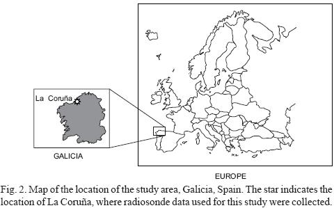
With data from Galicia (Spain) (Fig. 2) in the period 1993–2005, during summer months (from July to September), the GD model and the HI are applied. This is the main fire season in this region. Galicia reaches a maximum elevation over the sea of 2127 m. The complete fire database includes 70,000 fires, in which the annual average daily fire risk (DFR) was assessed. Values of the GD and the HI components were obtained from 0000 UTC radiosondes measurements at La Coruña, Spain.
We define NDFRi of a season of fire during a given period of study as the normalized value of DFR(i) for each type of day (i), defined as:
 , (4)
, (4)
(i = I, II, III and IV)
where ( ) is the average value of all seasonal DFRs (i) during the period of study, being i the type of day. Each seasonal value of DFR(i) is defined as the number of fires in days of type i, in a given season of fire, divided by the number of days of type i in this season on which fires occurred. The NDFR must be interpreted as an intrinsic proportion of risk for each type of day.
Since the GD model was originally developed using fire data from the period 1985–1994, this new data provides an evaluation test for the model.
Different statistical analysis (ANOVA of one factor, post hoc DMS and ANOVA with one covariable) are used in order to support the results of DFR obtained in this work.
3. Results
Table II and Figure 3 show the results of analysis when days are classified as type I, II, III, or IV, according to the GD model. Note that the DFR increases from type II to type I, following the sequence II–IV–III–I. In terms of humidity alone, risk increases from moist (types II and IV together) to dry (types I and III together). More interesting results appear when the influence of stability is analyzed. As can be seen, this sequence is clearly crossed. Under dry conditions (types I and III), when low stability exists, an increase of fire activity is produced, whereas under moist conditions (types II and IV), when low stability exists, a decrease of fire activity is produced. Therefore, only low stability increases fire activity on dry days.
In order to support these affirmations a statistical analysis has been made. In an ANOVA of one factor, in which type is an independent variable and DFR is a dependent variable, it has been obtained the following result: F(3.48) = 35.858; p < 0.001. This result indicates that there are significant differences between DFRs. In a probe post hoc DMS it has obtained the following results: between type I and II differences were significant (p < 0.001), between type I and III differences were not significant (p < 0.086), between I and IV differences were significant (p < 0.001), between II and III differences were significant (p < 0.001) and between II and IV differences were significant (p < 0.001). In an ANOVA in which type is an independent variable, DFR is a dependent variable and year is covariable, it has been obtained the following results: A significant effect in variable type (p < 0.001; eta = 0.692). The high value of the effect indicates that the differences between types are very clear. Moreover, these differences are maintained along years because the covariable year has not a significant effect (p = 0.880; eta < 0.001).
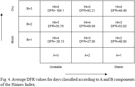
Table III and Figure 4 present results of the HI. Observe that the highest DFR is obtained for unstable and dry conditions (A = B = 3). Until here the coherence with the GD is shown. However, in the rest of the variants, the pattern that relates DFR with stability and moist conditions is not maintained. For low or intermediate stability (A = 2 or 3) DFR is inversely related to humidity, while for high stability (A = 1) the highest DFR corresponds to intermediate humidity. For low humidity (B = 3) DFR is inversely related to stability, while for high humidity (B = 1) DFR is proportional to stability. For intermediate humidity (B = 2) DFR is highest in intermediate stability.
Statistically, an ANOVA of one factor with DFR as dependent variable and type as independent value show following result: F(8.108) =10.049, p < 0.001. p indicates significant differences between classes. In a probe post hoc DMS results about the relation between different types each other have been obtained (Table IV). In a 41.6% of the possible combinations there were no significant differences (p > 0.05). For example between very low type (A = 1, B = 2) and moderate type (A = 3, B = 2) p = 0.824. In ANOVA with one covariable in which DFR is dependent variable, type is independent variable and year is covariable, a significant effect in type variable have been obtained (p < 0.001; eta = 0.429). These values indicate significant differences between types. With respect to year variable, there is no significant differences (p = 0.301; eta = 0.010). Therefore the differences are maintained along years. Nevertheless it would be needed to take more observations in order to obtain more conclusive results.
4. Discussion
According to the GD model results of Table II and Figure 3, if humidity is assumed as the primary factor for determining fire activity, stability plays a very important role as an authentic regulator of the fire occurrence. Whereas in the dry domain the low stability increases the number of fires, a drastic reduction is observed in the moist domain.
These results indicate that confusing results will be produced by mathematical addition of instability and dryness measures. In a supposition of the GD model like a simple addition of terms, the maximum value of addition (maximum risk) would be accurately presented in type I (low humidity and low stability), while the minimum value (minimum risk) would be expected for type IV (high humidity and high stability) days, although the results do not indicate this. Results are similarly inaccurate for crossed conditions of instability and humidity –high humidity and low stability or low humidity and high stability.
Statistical results support these affirmations. Results of an ANOVA of one factor indicate that there are differences in DFR depending of the type. But it is necessary to know differences between four types each other and for that a probe post hoc DMS has been carried out. In this study results indicate that in all cases differences were significant except for types I and III. We must remind that I and III are types of maximum risk of fire. A mistake of definition of type between I and III have not important consequences in management. Although in the rest of cases are perfectly distinguishable. For example between types I and II days have significant differences, thus, there is not risk of false alarm or under prediction. The objective of the last ANOVA with year as covariable have been to know if the differences between types and if risk of fire are maintained along years. Results were successful and indicate that DFR can be used in order to define risk of fire not only in a concrete year, along different years as well.
In view of the HI results of Table III and Figure 4, the consequences of adding the A and B components of the HI should be considered. Overall for the HI, the average DFR values increase with increasing index value (Fig. 4). Although, some DFR of the three combinations of A and B that yield a HI = 4, is lower than some DFR for HI = 2, or is greater than some DFR for HI = 5.
ANOVA of one factor indicate that in HI there are differences between types. Initially this is a good result for HI as system to detect fire risk levels. But in a probe post hoc DMS (Table IV) is proved that many relationships between types are very similar. There are not almost statistical differences between very different types operationally and it can cause important mistakes in fire management. For example if one day is defined with very low risk because A = 1 and B = 2, can be really a day with moderate risk (A = 3, B = 2). (p between these types shows high similarity). This is a clear case of underprediction. The most important thing in a system to detect risk of fire is that it could correctly define each class and if there is any possibility of mistake at least it must not have bad consequences in management. Moreover, ANOVA with year as covariable indicates that the before results are maintained along years, and therefore, mistakes in management can be presented in similar form year to year.
If in the GD model there was an additional scheme similar to the HI, combinations corresponding to moderate risk (types II and III) would form a single category, and its average DFR would be between the DFR for types I and IV. But in fact, the average DFR types II and III are really quite different. Moreover, the average DFR of type IV is intermediate between them. The addition of the components of stability and humidity causes a substantial loss of information that could be of great importance to fire management in forest fires.
A wild land fire is a vertical process and, consequently, must be connected with the vertical structure of the local atmospheric column. This matter has been established in published studies by many authors. Atmospheric instability, according to results presented here, has shown a dual effect on fire activity. Under dry conditions fire activity is increased by instability, but under moist conditions it is decreased. In essence, instability enhances the effect of dry or moist air in fire activity, while stability reduces such an effect.
For humidity and stability the results shown in this work make physically sense. Fire data analyzed here are about occurrence, not fire intensity or spread rate. Occurrence of fires is dependent of the flammability of fine fuels, which is primarily dependent of moisture content (Baeza et al., 2002; De Luis et al., 2004). If air is under moist conditions, it will not dry fuels, in fact it can even make them wet, thus, reducing fire risk. If air is dry, it will eliminate the water content of fuels, and therefore increase fire risk. On the other hand, while atmospheric stability impedes vertical circulation in the atmosphere, weak stability and instability not. In low stability conditions a larger volume of air to the ground is brought to upper levels by turbulence and vertical mixing, which favor a renovation of air around the initial ignition point. This fact permits the contribution of oxygen to the combustion reaction.
This paper points out several contradictions that arise in current fire risk indices. Analysis of data using the GD model, which use stability and humidity separately and does not seek to combine them mathematically, provides a clear demonstration of the true relationship between both parameters in fire activity. An analysis of the HI illustrates that stable and moist days (the lowest risk category for the Haines Index) do not correspond to the minimum value in DFR. As result of the addition of the A and B terms in the HI, different levels of fire risk are observed for the same value of the index. Although the HI presents positive results in unstable and dry days. According to the direct combination of the separate effects of instability and humidity, the HI correctly detect the most dangerous days, but not days with the lowest and the intermediate danger.
In the introductory section of this paper, several properties for suitable index were listed: briefly, clear correspondence, consistency with scientific knowledge, and no ambiguity. According to results, the GD index has all of them. Day type clearly corresponds to daily fire risk. Moreover, the separate day types do not contain any ambiguity about the conditions represented.
Although, analyzing the HI these properties are not taken into account. The HI does not show clear correspondence with DFR. Certainly, the highest value of the index corresponds with the highest DFR, but the lowest value of the index with the lowest DFR does not. The incorporation of stability and humidity to the index is consistent with atmospheric physics and wildland fire science, though the addition of the two values is not physically motivated. The Haines Index is ambiguous as applied here, and so fails to get the last criterion. Addition of the stability and humidity components produces identic result for very different situations about risk of fire, and can become misleading.
As noted earlier in this paper, the HI was designed for use with large fires under low wind conditions. Although, according to results observed in this paper, the HI shows strong correspondence with data set of many smaller fires, as well. Therefore, conditions of the atmospheric column substantially influence in superficial fire activity in all sizes of fires. The ambiguity in results of the HI was not produced by data set use; otherwise by the design of the index. Other authors, such as Potter (2003) and Jenkins (2004) include concepts CAPE and CIN that are common in theoretical studies of cumulus or convective development. This is physically appropriate, but the physical proprieties of the dry static energy, S, and moist static energy h, may be easily connected with CAPE and CIN.
This study further served to confirm the earlier results found for the GD model, using an independent data set. The progression of increasing DFR was II–IV–III–I, as in García Díez et al. (1994a).
Acknowledgement
Thanks to a research grant of Universidad de Salamanca and a project of Castilla y León (Spain) government, this study has been possible.
References
Arakawa A. and W. H. Schubert, 1974. Interaction of a cumulus cloud ensemble with the large–scale environment. Part I. J. Atmos. Sci. 31, 674–701. [ Links ]
Baeza M. J., M. de Luis, J. Raventós and A. Escarré, 2002. Factors influencing fire behaviour in shrublands of different stand ages and the implications for using prescribed burning to reduce wildfire risk. J. Environ. Manage. 65,199–208. [ Links ]
Chunmei X., M. Yousuff Hussaini, P. Cunnigham, R. Rodman and S. L. Goodrick, 2003. Numerical study of effects of atmosphere temperature profile on wildfire behavior. Proceedings of the 5th Symposium on Fire and Forest Meteorology, Paper J2.3 in 17–20 November, Orlando, Florida. American Meteorological Society. [ Links ]
Crosby J. S., 1949. Vertical wind currents and fire behavior. Fire Control Notes 10, 12–14. [ Links ]
de Luis M., M. J. Baeza, J. Raventós and J. C. González–Hidalgo, 2004. Fuel characteristics and fire behaviour in mature Mediterranean gorse shrublands. Int. J. Wildland Fire 13, 79–87. [ Links ]
Flannigan M. D. and J. B. Harrington, 1988. A study of the relation of meteorological variables to monthly provincial area burned by wildfire in Canada. (1953–80). J. App. Meteorol. 27, 441–452. [ Links ]
García Díez E. L., L. Rivas Soriano, F. de Pablo Dávila and A. García Díez, 1994a. An objective model for the daily outbreak of forest fires based on meteorological considerations. J. Appl. Meteorol. 33, 519–526. [ Links ]
García Díez E. L., L. Rivas Soriano, F. de Pablo Dávila and A. García Díez, 1994b. Objective method for the daily prediction of the number of forest fires. Proc. 2nd International Conference on Forest Fire Research. University of Coimbra (Portugal), II, 759–765. [ Links ]
García Díez A., L. Rivas Soriano and E. L. García Díez, 1996a. Medium–range forecasting for the number of daily forest fires. J. App. Meteorol. 35, 725–732. [ Links ]
García Díez A., L. Rivas Soriano, F. de Pablo Dávila and E. L. García Díez, 1996b. Spatial validity of a forecast model for the daily number of forest fires: Statistical analysis. Int. J. Biometeorol. 39, 148–150. [ Links ]
García Díez A., L. Rivas Soriano, F. de Pablo Dávila and E. L. García Díez, 1996c. Statistical analysis for the spatial validity of a model to forecast the daily number of forest fires. Int. J. Biometeorol. 39, 148–150. [ Links ]
García Díez E. L., L. Rivas Soriano, F. de Pablo Dávila and A. García Díez, 1999. Prediction of the daily number of forest fires. Int. J. Wildland Fire 9, 207–211. [ Links ]
Haines D. A., 1988. A lower atmosphere severity index for wildland fires. National Weather Digest 13, 23–27. [ Links ]
Jenkins M. A., 2002. An examination of the sensitivity of numerically simulated widfires to low–level atmospheric stability and moisture, and the consequences for the Haines Index. Int. J. Wildland Fire 11, 213–232. [ Links ]
Jenkins M. A., 2004. Investigating the Haines Index using parcel model theory. Int. J. Wildland Fire 13, 297–309. [ Links ]
McArthur A. G.,1996. Weather and grassland fire behavior. Commonwealth of Australia. Department of National Development. Forestry and Timber Bureau. Leaflet Number 100, Camberra. Australian Capital. [ Links ]
Potter B. E., 2002. A dynamics based view of atmosphere–fire interactions. Int. J. Wildland Fire 11, 247–255. [ Links ]
Potter B. E, Goodrick, S. L. and T. J. Brown, 2003. Development of a statistical validation methodology for fire weather indices. AMS Symposium on Fire and Forest Meteorology. (2003–5FIRE), 5. [ Links ]
Reifsnyder W. E., 1977. A fire rating system for the Mediterranean region. FAO/UNESCO Technical Consultation on Forest Fires in the Mediterranean Region. Forestry Dept. 9. [ Links ]
Taylor R. J., D. G. Corke, N. K. King, D. A. MacArthur, D. R. Packham and R. G. Vines, 1971. Some meteorological aspects of three intense forest fires. Division of Meteorological Physics Technical Paper 21. CSIRO, Australia. [ Links ]
Taylor R. J., S. J. Evans, N. K. King, E. T. Stephens, D. R. Packham and R. G. Vines, 1973. Convective activity above a large–scale bushfire. J. Appl. Meteorol. 12, 1144–1150. [ Links ]

