On a more consistent definition of radar reflectivity

 

R. FRAILE and M. FERNÁNDEZ–RAGA
Departamento de Física, Facultad de Ciencias Biológicas y Ambientales (IMARENAB)
Universidad de León, León, España
Corresponding author: R. Fraile; e–mail: roberto.fraile@unileon.es

 

Received October 26, 2008; Accepted September 8, 2009

 

RESUMEN

Se ha demostrado que la medida del factor de reflectividad del radar como 10 log₁₀ Z adolece de cierta inhomogeneidad, al no ser adimensional el argumento del logaritmo. En consecuencia, la medida en dBZ depende de las unidades utilizadas para medir Z. En su lugar, se propone una expresión del tipo 10 log₁₀ (Z/Z₀). Una elección adecuada de la constante Z₀ (10^–18 m³) hará que esta redefinición no afecte a las medidas realizadas y publicadas hasta la fecha, pues el resultado en dBZ será exactamente el mismo. Se ha intentado buscar un significado físico a Z₀ en relación con los parámetros característicos de la lluvia. Podría ser un indicador de la precipitación mínima apreciable registrada en un día, pero esto no puede extrapolarse a todos los tipos de precipitación. Sin embargo, sí se puede afirmar que, para una distribución concreta de tamaños de hidrometeoros, proporciona una referencia física en términos del número y volumen de las gotas de lluvia.

 

ABSTRACT

Measuring radar reflectivity as 10 log₁₀ Z is inhomogeneous, since the argument of the logarithm is not dimensionless. Consequently, measurements in dBZ depend on the units used to measure Z. This study, in contrast, suggests an expression of the type 10 log₁₀ (Z/Z₀). An adequate selection of the constant Z₀ (10^–18 m³) will produce a redefinition that will not affect the measurements that have already been carried out and published up to now, since the result in dBZ will remain unchanged. A physical meaning has been searched for Z₀ in relation with parameters typical for rain. It could be considered as an indicator of the minimum daily precipitation, but this cannot be extrapolated to all types of precipitation. However, it may be affirmed that for a specific distribution of hydrometeor sizes, Z₀ provides a physical reference in terms of the number and volume of raindrops.

Keywords: Precipitation, Z–R relation, Marshall and Palmer distribution.

 

1. Introduction

A meteorological radar is an active instrument of teledetection which operates on the basis of the emission and reception of electromagnetic waves in the range of microwaves. The microwaves cover the electromagnetic spectrum from 10^–1 to 10³ GHz, although the most commonly used radar frequencies lie between 1.5 (L–band) and 94 GHz (W–band). Frequency is a physical variable applicable exclusively to waves, unlike wavelength λ which depends also on the medium index of refraction n. In the atmosphere (n ≈ 1) the wavelengths which correspond to the radar frequencies mentioned above lie between 0.3 and 20 cm.

Radiation, when emitted to the atmosphere, interacts with cloud systems and a small amount of the energy is backscattered by the target and then detected by the radar. The analysis of the difference between the radiation released and the one received provides physical information about the meteorological target. The so–called meteorological radar equation represents the averaged power P_r measured by an antenna which can be expressed as:

where the constant C depends on the technical characteristics of the radar, r is the radar–target distance, L represents the attenuating features between the radar and the target, and η is called reflectivity. This variable is a function of the number N of the scattering elements per volume unit inside the cloud and of their physical properties. As a result, the power detected depends on the characteristics of the radar, the target and also on the medium between them.

Under the Rayleigh (1871) approximation, a new variable Zmay be defined called reflectivity factor so that:

where K is a constant that depends on the units used. In fact, in radar meteorology, the useful variable is the equivalent reflectivity factor Z_e, which is the reflectivity of a spherical liquid hydrometeor satisfying Rayleigh's approximation and backscattering a signal of the same power as that which is effectively backscattered. Indeed, the nature of the hydrometeors inside the volume of resolution is in general not known. In this context, η = Kλ^–4Z_e. For practical reasons, Z_e is symbolized by Z and called reflectivity factor or simply reflectivity for the purposes of brevity (and perhaps because the term factor is not an appropriate name, instead of coefficient).

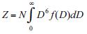
It is well known that the reflectivity factor of a number N of scattering elements per volume unit inside a cloud with size D_i is:

In fact, because hydrometeors are not perfectly spherical in shape (Brandes et al., 2002), size D_i is the equivalent diameter of a sphere that occupies the same volume as the hydrometeor considered. If N elements are classified into N' different classes (index j), each of them having nj hydrometeors of size D_j, the equivalent reflectivity factor is:

Finally, in continuous form, if n(D) is the number of scattering elements per unit of volume and size, then:

where the integral extends to all the sizes (equivalent diameters) of the elements. In other words, the integration extends from the minimum diameter to the maximum one. However, from a technical point of view, if the analytic form of n(D) is known, it can be easier to calculate the integration between 0 and infinity. Accepting this implies the possibility of ignoring the value of this integral between 0 and the minimum diameter, and between the maximum diameter and infinity. In any case, taking the integration limits from one side or the other does not have any influence on the aim of this paper, so this issue will not be discussed here any further.

From the relations described above it may be implied that, under the Rayleigh approximation, the reflectivity factor Z is independent of wave frequency: it depends exclusively on the number of scattering elements and their sizes. In other words, the reflectivity factor Z is a typical feature of the target. Because of this, this variable is generally preferred to reflectivity η, and it is also used more often.

The reflectivity factor Z is one of the most widely employed radar–related variables. Nearly all useful parameters such as water content or precipitation rate actually derive from the equivalent reflectivity factor. It is also very frequent to search for relations between Z and these parameters. These relations reveal the type of hydrometeor and the convective or stratiform nature of precipitation.

However, the reflectivity factor Z may take on values over about 10 orders of magnitude. Thus, a logarithmic scale is used for Z. This change in the scale is to blame for a certain inhomogeneity which will be the focus of this study.

 

2. A consistent definition of reflectivity factor

Reflectivity factor Z shows a wide range of variation. In the case of severe precipitation, for example hail, Z generally takes on values of 30,000 mm⁶ m^–3 and more, although there are registered cases of hail with Z values of around 4,000 mm⁶ m^–3 (Castro et al., 1992; Fraile et al., 2001; Fernández–Raga et al., 2009). Values over 100,000,000 mm⁶ m^–3 most probably correspond to large solid obstacles and not to precipitation. On the other limit of the scale, Pujol et al. (2007) have found Z values as low as 0.00001 mm⁶ m^–3 in warm clouds.

This wide range of values has resulted in the use of a logarithmic scale, which permits to contract the scale and, therefore, is more manageable for practical purposes. A traditional definition of the reflectivity factor (Battan, 1973; Rogers and Yau, 1989; Sauvageot, 1992; Rinehart 1997; and many others) reads as follows:

10 log Z,

measured in dBZ. Here, and in the rest of the article, the term "log" refers to the logarithm function in base 10.

From the point of view of dimensional analysis, this definition is not consistent because of the dimension of Z (L⁶ L^–3 = L³, where L is length). The application of the logarithmic function (like for trigonometric functions, or the exponential one) requires a dimensionless argument. As a consequence, the result depends on the units chosen for Z. This does not seem to be a practical problem, as in the radar literature Z is always measured in mm⁶ m^–3, so that many authors seem to comply with this formal inhomogeneity.

Nonetheless, the inhomogeneity of the logarithmic definition of the reflectivity factor is not taken into account when establishing other definitions related to the first. For example, Pujol et al. (2005) use differential reflectivity as:

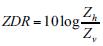
where Z_h and Z_v are the horizontal and vertical reflectivities, respectively. These same authors use the linear depolarization ratio as:

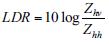
where Z_hv and Z_hh are the vertical and horizontal reflectivities of the backscattered signal, whereas the incident radar wave was horizontally polarized. In both definitions the coherence is respected since the numerator and the denominator have the same dimensions.

Bearing this in mind, we suggest a redefinition in order to re–establish the coherence of the equality, as is done for studying, for example, sound waves and the intensity expressed in decibels (Alonso and Finn, 1992). A more accurate definition would be:

Of course, to preserve the numerical results obtained with the classical definition, the value for Z₀ must be 1 mm⁶ m–³. This value for Z₀ is 1 mm³, or, in the International System of Units,

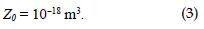
This redefinition puts reflectivity decibels (dBZ) on the same level as the other decibels used in scientific literature. From the Weber–Fechner Law, which relates the magnitude of a physical stimulus to its perception (Fechner, 1860), it became more common to use the logarithmic scale to measure variables taking on values of several orders of magnitude.

Today many variables are commonly measured on a logarithmic scale, particularly in decibel: power, intensity, amplitude, gain, noise, etc., in many different fields of physics, such as optics, acoustics, electronics and other technological applications. Even other scales, such as the Richter (1935) scale, which quantifies the seismic energy released by an earthquake, is also logarithmic, although it does not use the decibel as the unit of measurement. In any case, all these scales express the magnitude of a physical variable in relation to a reference level, i.e., they all take the form of the logarithm of a dimensionless fraction whose denominator is precisely the reference established. The idea put forward here is to maintain homogeneity in the measurements of radar reflectivity.

 

3. Interpretation of Z₀

As stated above, Z and Z₀ have volume dimensions. In fact, the values mentioned for hail (45 dBZ) and for obstacles (80 dBZ) represent reflectivities of about 3 x 10^–14 m³ and 0.1 mm³, respectively.

Clearly, Z₀ can be called the reflectivity factor threshold (which is also a volume threshold), because, for a radar resolution volume, when Z = Z₀, the logarithmic value is zero, and when Z< Z₀ the amount in (1) takes on negative values.

Writing the reflectivity factor Z in a continuous form, i.e. when N is the total number of drops per unit of volume and f (D) is the probability density function (PDF) it reads as follows:

which is equivalent to substituting n(D) in Equation (1) for N f (D). Considering a Marshall and Palmer (1948) (hereinafter referred to as MP) exponential distribution, and taking the PDF as f (D) = βe^{– βD} (Fraile and García–Ortega, 2005), parameter Z is:

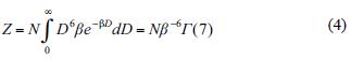
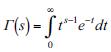
where Γ is the factorial or Euler gamma function, defined as:

What represents the value Z₀ in Equation (3)? What does it physically mean? From Equation (4), when the value of Z is Z₀, the number (or, better, the concentration) N of drops is only a function of β, as can be seen in Figure 1. Parameter β has some peculiar features: it is always positive and its dimensions are L^–1, so that the argument of the exponential function is dimensionless. In addition, because the PDF is normalized, β represents simultaneously the value that the PDF has at the beginning and the speed of its drop.

There are different ways to calculate β (Fraile et al., 2009). The values of β corresponding to the most frequent precipitation intensities R (mm h^–1) are represented on the abscissas of Figure 1. This has been done on the basis of the most common β – R relations, which are of the type β = AR^B. The traditionally accepted values of the parameters are A = 41 cm^–1 (mm h^–1)^–B and B = –0.21 (Marshall and Palmer, 1948). However, the literature mentions values of A ranging from 30 in the case of storms (Joss et al., 1968), and even from 27 (Benett and Fang, 1984), to 57 for drizzle (Joss et al., 1968). As for B, the range of values lies between –0.258 (Uijlenhoet and Stricker, 1999) and–0.21.

With the values of A and B mentioned above we may obtain the approximate range of β for the various precipitation intensities. If we considerthe two extremes of precipitation intensity, we have R = 0.1/24 mm h^–1 (that is, 0.004 mm h^–1, which is a negligible intensity of rain) as the minimum value. To determine a maximum value of R we have checked the records of intensities published by Galmarini et al. (2004) and by Dunkerley (2008), who report several cases of intensities higher than 500 mm h^–1. The absolute maximum is over 2,000 mm h^–1 during one minute. This value was registered on November 26, 1970 in Guadalupe. In these cases, the β values range between 380 and 23,000 m^–1. This range of values comprises the interval between 1,330 and 4,300 m^–1, which is the most frequent, according to Coutinho and Tomás (1995).

The area under the curve in Figure 1 represents the condition Z < Z₀: the reflectivity factor defined according to Equation (2) takes on negative values in that region.

Equation (4) provides different possibilities for relating the variables Z, β and N. For example, for a given value of β, when Z = Z₀, the result is that Z₀=N₀/T F(7), so, using Equation (2) Z = 10 log (N/N₀). In this case, Z₀ is the equivalent reflectivity factor of a given number (N₀) of hydrometeors. Therefore, it may be seen directly that if N > N₀, Z > Z₀ and if N < N₀, Z < Z₀. Another possibility is to fix N and determine the corresponding value of β. In this case, it would also be possible to refer to a β₀.

All of the possible relations between the three variables are displayed in Figure 2. Here we may see the surface of Equation (4), namely Z as a function of β and N. One can use for example a relation between Z and β for a given value of N. The figure shows the curve corresponding to N = 100 dm^–3, which is one of the limits of the surface. Another example is that of the curve Z = Z₀ which according to Equation (2) is equivalent to the line of 0 dBZ, indicated with a thicker line).

Another interesting question refers to the volume Vof liquid water represented by Z₀. Considering that drops follow the MP distribution, the volume of liquid water per unit of volume of air is the integral of f (D) multiplied by the volume of each drop, that is,

Figure 3 represents the liquid water content (LWC: mass of liquid water in the unit of volume of air) as a function of the concentration N of drops when the reflectivity factor for the sampled volume is Z₀. The curve of Figure 3 is a square root, since taking Equation (4) for Z = Z₀:

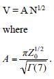
Over the curve in Figure 3, the reflectivity in that parcel will be Z > Z₀ and the reflectivity factor defined as in Equation (2) will be positive.

The representation of the LWC as a function of β is shown in Figure 4 in logarithmic scales. As in the previous figures, to the left of the line we have Z > Z₀ and the reflectivity factor defined as in Equation (2) will also be positive.

Finally, the relation between Z₀ and the precipitation intensity was analyzed. In studies carried out with meteorological radar it is common to make use of empirical relations extracted from the scientific literature (Blanchard, 1953; Jones, 1956) to estimate the precipitation intensity. Again following MP, we establish a relation Z–R as:

Z=200 R^1.6

where R is the precipitation intensity in mm h^–1 and Z the reflectivity in mm⁶ m^–3.

Because Z₀ = 1 mm⁶ m^–3, the value of the associated precipitation intensity will be R = (1/200)^1/1.6 = 0.036 mm h^–1, which for a whole day is less than 1 mm (more precisely 0.875 mm).

In radar meteorology the MP relation is not the only employed. In the past twenty years or so, many other relations have been suggested. For example, Uijlenhoet and Stricker (1999) have warned against the inconsistency of the MP relation and have obtained a different one using the same hypotheses. Lee et al. (2007) have found in a storm in Canada the relation Z = 206 R^1.55, even though the climatologic relation in Montreal is Z = 210 R^1.47. Comstock et al. (2004) have claimed that the exponent of R may vary between 1 and 1.5 (they also found a value of 0.9). Lee et al. (2004) have found for this parameter an interval from 1.65 to 2.08 for stratiform rain (Z = 366 R^1.75) and from 1.20 to 1.42 for convective rain (Z = 414 R^1.35). Finally, Lee and Zawadzki (2005a, b) have reviewed the variability of Z–R relations by presenting the various values taken on by these two parameters.

Taking into account the extreme values obtained by the authors mentioned above, it may be said that the precipitation intensity associated to a reflectivity of Z₀ lies between 0.006 and 0.06 mm h^–1, which would amount to a total daily precipitation (24 h) of slightly over 0.1 and 1.5 mm. This is, of course, a very small amount. However, we may not state as a fact that Z₀ represents the reflectivity factor threshold for negligible daily precipitation because this depends on the most adequate Z–R relation for each type of precipitation.

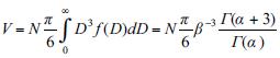
Raindrop size distribution is not always exponential. It is often the case, especially in small sizes, that there are actually fewer drops than expected. Instead of the MP exponential distribution it is therefore possible to use the gamma distribution, a well–known alternative in the case of raindrop size distributions (Ulbrich, 1983; Brawn and Upton, 2008a), with f (D) = β^α D^α–1 e^–βD/ Γ(α) (Fraile et al., 1999). It was found that when α = 1 the gamma distribution turns into an exponential distribution.

With a gamma distribution, parameter Z will be, like Eq (4):

Following the same argumentative line as in the case of the PM distribution, it is easy to determine that with the gamma distribution the volume of liquid water will be:

so that for Z = Z₀ it is again true that V=A' N^1/2 although now

In these three last equations the same form as the one found for the MP distribution is maintained, except in one factor which depends on parameter a of the gamma PDF.

To estimate the differences between the two distributions we used the values of a which Brawn and Upton (2008b) used to describe seven categories of rainfall. In these categories a takes on values between 1 and 9.9. In the higher values of a (extreme rain events) Nmight grow three orders of magnitude with respect to the curve shown in Figure 1. At the same time, considering a gamma distribution implies that Vmay grow two orders of magnitude with respect to what was computed for the MP distribution. Finally, A' may triple the value of A in the case of values of a close to 10.

This strong dependence on the raindrop size distribution does not support a physical significance for Z₀ in the style of the threshold intensity of the Weber–Fechner Law. However, Z₀ provides a physical reference in terms of N or V for a given hydrometeor size distribution. This is exactly the same as for acoustics or filters in electronics, for instance. The value of Z₀ has been put forward for practical reasons. A different value of Z₀ may have been selected with clearer meteorological uses. The problem is that it does not seem to be easy to achieve its acceptance on the part of the scientific community after several decades employing a widely–used, though inconsistent, system.

 

4. Discussion and conclusions

The main conclusion that can be drawn from this study is the proposal that the measurement of the radar reflectivity factor as 10 log Z should not be used in this way since the argument of the logarithm is not dimensionless, and, therefore, the result depends on the units used to measure Z. Using specific units to keep up an inhomogeneous equation is not a solution. We believe that dimensional formalism is an important part of physics, facilitating not only the computation but also the assimilation of concepts. So, homogeneous relations should be used whenever possible. Therefore, in this case we suggest the expression 10 log (Z/Z₀), where Z₀ has the same dimensions as Z. Simultaneously, we suggest that Z₀ = 10^1–8 m³.

From a practical perspective, this redefinition does not affect results, since the logarithm has traditionally been applied onto a value of Z measured in mm⁶ m^–3. The value of Z₀ has been selected in such a way as to avoid variation with the value of the reflectivity factor which has traditionally been measured in dBZ.

Finally, the value of Z₀ was not found to represent any significant threshold from a physical point of view, out of the reflectivity of 1 mm diameter drop in 1 m³. In any case, it could represent in very specific circumstances the minimum daily precipitation registered, but this cannot be made extensive to all types of precipitation. The main significance of Z₀ is to provide a physical reference according to the quantity of hydrometeors and their volume, for a distribution given in hydrometeor sizes.

In contrast with the definitions of decibel starting from perceptions (such as the above mentioned Weber–Fechner Law, where the reference constant is a perception threshold), the definitions based on units (such as dBZ) take as a reference a certain unit of measurement with the only aim of simplifying the expression of the measurements.

It would have been interesting to suggest the redefinition of dBZ with a value of Z₀ chosen so as to be a characteristic threshold. However, after many years using one particular scale, it would be rather pretentious that the authors attempt to challenge and modify the value of Z₀ used by the scientific community, implying a complete change in the scale of measurement. This is not the aim of this study. The suggestion of a new definition with a higher mathematical coherence is sufficiently relevant.

 

Acknowledgements

The authors wish to express their thanks to Dr. Noelia Ramón for the translation of this paper into English and to Dr. A. Castro for her suggestions. The authors are also grateful to the three anonymous reviewers for their useful comments. This study was supported by CICYT (Grant TEC2007–63216) and the Junta de Castilla y León (LE014A07).

 

References

Alonso M. and E. J. Finn, 1992. Physics. Addison–Wesley Publishing Company, Wokingham. 156 pp.        [ Links ]

Battan L. J., 1973. Radar observation of the atmosphere. University of Chicago Press, Chicago.        [ Links ]

Benett J. A. and D. J. Fang, 1984. The relation between N₀ and L for Marshall–Palmer type raindrop–size distributions. J. Climate Appl. Meteor. 23, 769–771.        [ Links ]

Blanchard D. C., 1953. Raindrop size distribution in Hawaiian rains. J. Meteor. 10, 457–473.        [ Links ]

Brandes E. A., G. Zhang and J. Vivekanandan, 2002. Experiments in rainfall estimation with a polarimetric radar in a subtropical environment. J. Appl. Meteor. 41, 674–685.        [ Links ]

Brawn D. and G. Upton, 2008a. On the measurement of atmospheric gamma drop–size distributions. Atmos. Sci. Let. 9, 245–247.        [ Links ]

Brawn D. and G. Upton, 2008b. Estimation of an atmospheric gamma drop size distribution using disdrometer data. Atmos. Res. 87, 66–79.        [ Links ]

Castro A., J. L. Sánchez and R. Fraile, 1992. Statistical comparison of the properties of thunderstorms. Atmos. Res. 28, 237–257.        [ Links ]

Comstock K. K., R. Wood, S. E. Yuter and C. S. Bretherton, 2004. Reflectivity and rain rate in and below drizzling stratocumulus. Q. J. R. Meteorol. Soc. 130, 2891–2918.        [ Links ]

Coutinho M. A. and P. P. Tomás, 1995. Characterization of raindrop size distributions at the Vale Formosa experimental erosion center. Catena 25, 187–197.        [ Links ]

Dunkerley D., 2008. Rain event properties in nature and in rainfall simulation experiments: a comparative review with recommendations for increasingly systematic study and reporting. Hydrol. Process. 22, 4415–4435.        [ Links ]

Fechner G.T., 1860. Elemente der Psychophysik. Breitkopf und Härtel, Leipzig.        [ Links ]

Fernández–Raga M., A. Castro, C. Palencia, A. I. Calvo and R. Fraile, 2009. Rain events on 22 October 2006 in León (Spain): Drop size spectra. Atmos. Res. 93; 619–635.        [ Links ]

Fraile R., J. L. Sánchez, J. L. de la Madrid, A. Castro and J. L. Marcos, 1999. Some results from the Hailpad Network in León (Spain): Noteworthy correlations among hailfall parameters. Theor.Appl. Climatol. 64, 105–117.        [ Links ]

Fraile R., A. Castro, J. L. Sánchez, J. L. Marcos and L. López, 2001. Noteworthy C–band radar parameters of storms on hail days in northwestern Spain. Atmos. Res. 59–60, 41–61.        [ Links ]

Fraile R. and E. García–Ortega, 2005. Fitting an exponential distribution. J. Appl. Meteorol. 44, 1620–1625.        [ Links ]

Fraile R., C. Palencia, A. Castro, D. Giaiotti and F. Stel, 2009. Fitting an exponential distribution: Effect of discretization. Atmos. Res. 93, 636–640.        [ Links ]

Galmarini S., D. G. Steyn and B. Ainslie, 2004. The scaling law relating world point–precipitation records to duration. Int. J. Climatol. 24, 533–546.        [ Links ]

Jones D. M. A., 1956. Rainfall drop–size distribution and radar reflectivity. Res. Rept. 6. Urbana: Meteor. Lab., Illinois State Water Survey.        [ Links ]

Joss J., J.C. Thams and A. Waldvogel, 1968. The variation of raindrop size distributions at Lacarno. Proc. Int. Conf. Cloud Physics, Toronto, AMS, 154–157.        [ Links ]

Lee G. W., I. Zawadzki, W. Szyrmer, D. Sempere–Torres and R. Uijlenhoet, 2004. A general approach to double–moment normalization of drop size distributions. J. Appl. Meteor. 43, 264–281.        [ Links ]

Lee G. W. and I. Zawadzki, 2005a. Variability of drop size distributions: Time–scale dependence of the variability and its effects on rain estimation. J. Appl. Meteor. 44, 241–255.        [ Links ]

Lee G. W. and I. Zawadzki, 2005b. Variability of drop size distributions: Noise and noise filtering in disdrometric data. J. Appl. Meteor. 44, 634–652.        [ Links ]

Lee G. W., A. W. Seed and I. Zawadzki, 2007. Modeling the variability of drop size distributions in space and time. J. Appl. Meteor. 46, 742–756.        [ Links ]

Marshall J. S. and W. M. K. Palmer, 1948. The distribution of raindrops with size. J. Meteor. 5, 165–66.        [ Links ]

Pujol O., J. F. Georgis, M. Chong and F. Roux, 2005. Dynamics and microphysics of orographic precipitation during MAP IOP3. Q. J. R. Meteorol. Soc. 131, 2795–2819.        [ Links ]

Pujol O., J. F. Georgis and H. Sauvageot, 2007. Influence of drizzle on Z–M relations in warm clouds. Atmos. Res. 86, 297–314.        [ Links ]

Rayleigh Lord, 1871. On the light from the sky, its polarization and colour. Phil. Mag. 41, 107–120.        [ Links ]

Richter C. F., 1935. An instrumental earthquake scale. Seismological Society of America Bulletin 25, 1–32.        [ Links ]

Rinehart R. E., 1997. Radar for meteorologists. Third edition. Rinehart Publications, Grand Forks, ND.        [ Links ]

Rogers R. R. and M. K. Yau, 1989. A short course in cloud physics. Third edition. Butterworth–Heinemann, Oxford.        [ Links ]

Sauvageot H., 1992. Radar Meteorology. Artech House. Boston, 384 pp.        [ Links ]

Uijlenhoet R. and J. N. M. Stricker, 1999. A consistent rainfall parameterization based on the exponential raindrop size distribution. J. Hydrol. 218, 101–127.        [ Links ]

Ulbrich C.W. 1983. Natural variations in the analytical form of the raindrop size distribution. J. Climate Appl. Meteorol. 22, 1764–1775.        [ Links ]