Calibration of the equations of Hargreaves and Thornthwaite to estimate the potential evapotranspiration in semi–arid and subhumid tropical climates for regional applications

 

F. BAUTISTA, D. BAUTISTA
Centro de Investigaciones en Geografía Ambiental, Universidad Nacional Autónoma de México
Antigua Carretera a Pátzcuaro Núm. 8701,
Col. Exhacienda de San José de la Huerta, Morelia, Michoacán
Corresponding author: F. Bautista; e–mail: leptosol@ciga.unam.mx

C. DELGADO–CARRANZA
Unidad de Recursos Naturales, Centro de Investigación Científica de Yucatán (CICY), Calle 43 No. 130, Col. Chuburná de Hidalgo, Mérida, Yucatán, México

 

Received September 28, 2008; Accepted August 20, 2009

 

RESUMEN

El método FAO Penman (PM), es el más confiable para estimar la evapotranspiración de referencia (ETo) y es recomendado por la FAO como estándar para verificar otros métodos empíricos. En su utilización es necesaria información de cuatro parámetros meteorológicos: temperatura del aire, humedad relativa, velocidad del viento y radiación neta. La poca disponibilidad de estos parámetros limita el uso del método en muchos lugares; por lo que los modelos Thornthwaite (TM) y Hargreaves (HM) son usados con frecuencia, ya que únicamente se basan en medidas de temperatura del aire, medidas comunes en muchas estaciones meteorológicas en todo el mundo, por lo que son una opción para estimar la ETo. Sin embargo, con el objetivo de obtener resultados apropiados de ETo, los modelos HM y TM deben ser calibrados de acuerdo con las condiciones locales. En el presente estudio, los coeficientes originales de TM y HM son modificados para una calibración local en climas semi–áridos y tropicales sub–húmedos del estado de Yucatán, México, usando como estándar la ecuación Penman–de FAO. Se usaron datos meteorológicos de dos estaciones en el estado de Yucatán, México que corresponden a un clima costero semi–árido (Progreso) y a un clima tropical sub–húmedo tierra adentro (Mérida). En la comparación se analizaron los índices de concordancia (D), confianza (C), correlación (R) y regresión (R²), así como indicadores del sesgo medio del error (MBE), raíz cuadrada media del error (RMSE), error relativo (RE) y el cociente entre ambas estimaciones promedio de ETo (r). Usando HM sin ajuste se obtuvieron buenas estimaciones de ETo en Mérida y Progreso, con valores de C de 0.825 y 0.816, respectivamente. No se recomienda el uso de TM sin ajuste en ninguna de las estaciones meteorológicas estudiadas. Sin embargo, en ambas estaciones, el modelo TM estima mejor la Eto durante los meses lluviosos (de junio a octubre). En ambas estaciones meteorológicas, costera y de tierra adentro, se obtuvieron mejores estimaciones anuales de ETo con el uso de HM sin ajuste (valores de C de 0.906 y 0.917, respectivamente).

 

ABSTRACT

The Penman–method (PM) to estimate the reference evapotranspiration (ETo) needs four meteorological parameters: air temperature, relative humidity, wind velocity, and net radiation, which may not be everywhere available and is the most reliable method and recommended by the FAO as the standard to verify other empirical methods. However, the Thornthwaite (TM) and Hargreaves (HM) models are frequently used because they are based on measurements of air temperature, commonly recorded in many meteorological stations throughout the world, becoming an option for estimating ETo. Nevertheless, in order to obtain appropriate results, the equations need to be locally calibrated. In the present study, the original coefficients of the TM and HM were modified for regional calibration in semi–arid and tropical subhumid in the state of Yucatán, México, using as a standard the Penman– equations of FAO. Meteorological data from two stations in the state of Yucatán, México were used, corresponding to a coastal, semi–arid climate (Progreso) and an inland, tropical subhumid climate (Mérida). In the comparison, the indices of concordance (D), confidence (C), correlation (R) and regression (R²) were analyzed, together with the mean bias error (MBE), root mean square error (RMSE), relative error (RE) indicators and the ratio between both average estimations of ETo (r). Using the HM without adjustment, we obtained good estimations of ETo, both in Mérida and in Progreso, with C values of 0.825 and 0.816, respectively. The use of TM without adjustment is not recommended in neither of the studied meteorological stations. However, in both stations, TM without adjustment is the best model for the estimation of ETo during the rainy months (from June to October). In both inland and coastal meteorological stations, better annual estimations of ETo are obtained by the use of the HM with adjustment (C values of 0.906 and 0.917 respectively).

Keywords: Calibration, evapotranspiration, Hargreaves, Thornthwaite, Yucatán, México.

 

1. Introduction

Information about evapotranspiration (ET), or consumptive water use, is significant for water resources planning, for irrigation scheduling in crops (Slabbers, 1977; Stefano and Ferro, 1997; Wu, 1997; García et al., 2007), and for forestry (Calder, 1977). Also, ET is very important for understanding natural plant communities (Monteith, 1964, 1965; Mielnick et al., 2005). As the changes of plant cover modify the ET and the energy balance, the knowledge and measurement of the changes in ET are necessary to understand the ecohydrological changes (Huxman et al., 2005; Cooper et al., 2006; Prater and DeLucia, 2006).

Potential ET is a function of atmospheric forcing and surface types. In order to remove the influence of surface types, the concept of reference evapotranspiration (ETo) was introduced to study the evaporative power of the atmosphere independent of crop type, crop development and management practices (Allen et al., 1998). This climatic parameter represents the evapotranspiration from a standard vegetated surface. As water is abundantly available at the reference evapotranspiring surface, soil factors do not affect ETo. Relating ETo to a specific surface (grass) provides a reference from which ET for other surfaces can be estimated (Doorenbos and Pruitt, 1977; Allen et al., 1998). In general, techniques for estimating ETo are based on one or more atmospheric variables, or on some measurements related to these variables, like pan evaporation. Some of these methods are accurate and reliable; others provide only a rough approximation.

The Penman–method (PM) is considered to be the most physical and reliable method and recommended by the FAO as the sole standard to verify other empirical methods (Allen et al., 1998). The FAO Penman– method has a strong theoretical basis, including energy balances to model ETo. It is based on fundamental physical principles, which guarantee the universal validity of the method. However, it needs four meteorological parameters: air temperature, relative humidity, wind, and net radiation, which may not be everywhere available (Smith et al., 1991; Allen et al., 1998; Camargo and Camargo, 2000).

Other methods only contemplate the temperature, as for example, those of Thornthwaite (1948) and Hargreaves (Hargreaves and Samani, 1982). These methods have the advantage of requiring few meteorological data; however, they were developed for use in specific studies and are most appropriately applied to climates similar to that where they were developed (Chattopadhyay and Hulme, 1997; Xu and Singh, 2000; Xu and Chen, 2005). In fact, large errors can be expected when these methods are extrapolated to other climatic areas without recalibrating the constants involved in the formulae (Hounam, 1971). Thornthwaite's model (TM) is very simple, only requiring mean air temperature, a widely available variable, and two tabular indexes: number of sunny hours, and monthly heat index (Thornthwaite, 1948). The TM is not recommended for use in areas that are not climatically similar to the east–central USA, where it was developed (Jensen, 1973). Hargreaves' model (HM) is a simpler model that requires only two meteorological parameters, temperature (mean, maximum and minimum) and incident radiation (Hargreaves and Samani, 1985). Although HM uses the extraterrestrial radiation (Ra) to estimate the ETo, for a given latitude and day, Ra can be obtained from tables or it can be calculated by means of a set of equations using temperature. Therefore, HM has become a temperature–based method (Xu and Singh, 2001).

In many regions of the planet, the meteorological stations do not have enough data to use PM. Therefore, it becomes necessary to develop procedures for realizing regional and temporal adjustments to HM and TM to obtain the best estimations of ETo (Rosenberg et al., 1983; Borges and Mendiondo, 2007). As well, numerous recalibration studies are also necessary, including case studies in different climatic regions so that the conclusions can be generalized (Xu and Singh, 2005).

In the Mexican state of Yucatán, only two meteorological stations have historical data for calculating ETo with PM, the remaining 38 stations in the state and neighbourhood only have data for calculating ETo using TM and HM.

The objectives of this study were to adjust the test equations (TM and HM) to the results of the reference model (PM) in semi–arid climate in a coastal locality (Progreso) and in tropical subhumid climate in an inland locality (Mérida) in the Yucatán Peninsula, México, in order to obtain two products: 1) identification of the test model with the best adjustment to the reference model (PM); and 2) to propose new values of constants (for month, season or year) for the models to be tested (HM and TM).

According to Xu and Singh (2001), this kind of studies remain to be justified by the fact that temperature–based evaporation calculation methods, although widely criticized, are still widely used and have often been misused because of their simple nature; these studies provide the best equation forms to users having only temperature data available.

 

2. Materials and methods

2.1 Study area

The data of three years (2001–2003) of the Mérida and Progreso meteorological stations in the state of Yucatán, México were used. Both meteorological stations have contrasting environmental conditions. In Mérida, the climate is tropical subhumid with annual mean temperature of 26.6 °C and 1173.5 mm of rainfall; the vegetation is of tropical dry forest. Mérida station is at 15 masl and is located inland. In the Progreso station the climate is semiarid with 32.9 °C of annual mean temperature and 511.2 mm of annual rainfall; the vegetation is a community of shrubs. The Progreso station, at an elevation of 2 masl, is located in the coast (Flores and Espejel, 1994; García, 2004). In the region under study are 40 weather stations, of which nine are in the neighboring states of Campeche and Quintana Roo (Fig. 1). Nine stations have a coastal environment and the remaining 31 have an influence on inland (Table I).

 

2.2 Description of the models for the estimation of ETo The estimation of ETo with PM uses the equation:

Where ETo is the potential evapotranspiration (mm d^–1); Δ is the slope of the saturation vapor pressure versus air temperature curve (kPa °C^–1); Rn is the daily net radiation (MJm–2d^–1); G is the soil heat flux (MJm^–2d^–1); y is the psychrometric constant (kPa^°C^–1); T_a is the daily mean temperature of the air at 2 m of height (°C); u₂ is the daily mean of wind speed at 2 m of height (m s^–1); e_s is the saturation vapour pressure (kPa); e_a is the actual vapour pressure (kPa) (Allen et al., 1998).

When estimating ETo fortime intervals less than a day, G may be neglected because its value is very small (Allen et al., 1998). However, fortime intervals greater than 1 day, for example a month, which is the time interval used in this work, the following equation (Allen et al., 1998) is used:

G_{month, i} = 0.14 (T_{month, i} T _{month, i – 1})

Where: G_month,i = Heat flux density in the soil during the month i (°C)

T_{month, i} = Mean air temperature of the month i (°C)

T_{month, i –1}= Mean air temperature from the previous month (°C)

Hargreaves (1975) made several regression analyses between measurements of various climate parameters and evapotranspiration. The regressions were made using a long series of combinations of climatic parameters. He found that for a period of 5 days, the temperature (°F) multiplied by Rs (global radiation at the surface) could predict 94% of the variance in the measurements of ET. Other parameters such as wind speed (U) and relative humidity (RH) only explained 10 and 9%, respectively. A subsequent analysis showed that Rs could be calculated with the extraterrestrial radiation (Ra) and the percentage of possible sunshine (S), also found that values of this last parameter averaged about five times those of the daily temperature range in °C. These were the facts that led to Hargreaves to derive the equation of the same name for the estimation of ETo (Hargreaves et al., 2003).

The estimation of ETo with HM is calculated by the equation:

Where ETo is the potential evapotranspiration (mm d^–1); T_max, T_min and T_med are the daily maximum, minimum and mean air temperatures (°C), respectively; Ci= 0.0023 is the original empirical constant proposed by Hargreaves and Samani (1985); and Ra is the water equivalent of the extraterrestrial radiation in mm d^–1 (Table II) (Hargreaves and Samani, 1985).

Due to air temperature is an important factor that transports water from the earth to atmosphere, Thornthwaite (1948) analyzed this parameter with data of evapotranspiration. He found that a general form of the relation can be: e = ctª

Where e, is the monthly evapotranspiration in centimeters and t is the mean air temperature in °C. The coefficients c and a vary from place and season. Thornthwaite proposed a general equation with a value of c = 16. Since the calculation of the evapotranspiration is not appropriate in areas with a monthly average temperature less than 0, an equation was developed to integrate this parameter, which corresponds to the monthly (i) and annual (I) heat index. Based on these, he proposed calculating the exponent a. Finally, an adjustment factor relating to the specific number of days per month and hours of sunlight, depending on the season and latitude is integrated to the equation (Thornthwaite, 1948).

The estimation of ETo with TM is computed in according with Thornthwaite (1948) by the equation:

Where ETo is the potential evapotranspiration (mm d^–1); ETo_sc is the gross evapotranspiration (without corrections); N is the maximum number of sunny hours in function of the month and latitude (Table II); dm is the number of days per month; C = 16 is a constant; I is the annual heat index; ais an exponent in function ofthe annual index: a = 0.49239 + 1792 x 10^–5 I – 771 x 10 ^–7 I² + 675 x 10^–9 I³; i is the monthly heat index; and tmed is the mean daily temperature (°C) (Thornthwaite, 1948).

The extraterrestrial solar radiation (Ra) and the maximum number of sunny hours have higher values from May to August and lesser values on November to January. In Progreso the values of extraterrestrial solar radiation are lower than in Mérida in the period from September to April (Table II).

 

2.3 Adjustment of models

The test estimations of ETo with HM and TM were adjusted to the result ofthe reference equation, that is PM. Adjustments were made by changing the value of the corresponding constant, Ci in the case of HM, and C in the case of TM, with the original values of 0.0023 and 16, respectively (Borges and Mendiondo, 2007).

The determination ofthe new values ofthe constants of HM (eq 2) and TM (eq 3) were calculated for each month ofthe three years of analyzed data.

Where: Ci_adj is the new value ofthe constant of Hargreaves; C_adj the new value of the constant of Thornthwaite; HM the monthly estimation of ETo with the equation of Hargreaves; TM the monthly estimation of ETo with the equation of Thornthwaite and PM the monthly estimation of ETo with the equation of Penman.

The average values ofthe constants ofthe tested equations were proposed by the annual variation ofthe new monthly value.

 

2.4 Comparison of models

The comparison of HM and TM with PM was carried out using a concordance index (D) (Willmott, 1982):

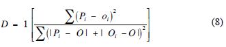
Where Pi is the value estimated for every model of test (TM and HM); O_i is the estimated values of PM; and O is the average of estimated values of PM.

The confidence index (C) was calculated by the product of the coefficient of lineal correlation (R) of the models by D.

C = 0 indicates null confidence and C = 1 indicates total confidence.

ETo estimates from both models (PM vs. HM and PM vs. TM) were compared using simple error analysis and linear regression. The models were compared before and after adjustment. For each location, the following parameters were calculated (Willmott, 1982): mean bias error (MBE), root mean square error (RMSE), relative error (RE) and the ratio between both average estimations of ETo (r).

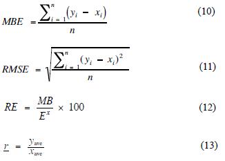
Where n is the number of available days; y_i is the ETo estimated with HM; x_i is the ETo estimated with PM; x_ave and y_ave are the averages for a given site of the ETo assessed by PM and of the ETo estimated by HM, respectively.

 

2.5 Regional news values of ETo

We calculated the ETo values of the 33 meteorological stations from Yucatán, we used the new coefficients of equations of TM and HM, considering the geographical position, coastal or inland from Progreso and Mérida, respectively. The effect of proximity to the coast or inland to estimate ETo has been widely reported (Gavilán et al., 2006; Martínez–Cob and Tejero–Juste, 2004).

In geomorphologic terms, the state of Yucatán is a karstic plain with elevations below 250 m, which suggests that the relief does not affect the air temperature.

We compare graphically the HM and TH with adjusted and non–adjusted data. We used the average data from 1961 to 2006. The sum of the differences between non adjusted and adjusted models was calculated (S) by monthly data for each meteorological station.

The S values are indicators of the overestimation or underestimation values of ETo with the values non adjusted.

 

3. Results and discussions

3.1 Comparison of ETo with three models without adjustment

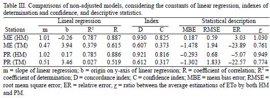
The linear regression models between PM and HM without adjustment present correlation values of R = 0.887 and R = 0.886 for the stations of Mérida and Progreso, respectively (Table III). The values of the concordance index are high (D = 0.93 and D = 0.92), as are the values of the confidence index (C = 0.825 and C = 0.816) forthe stations of Mérida and Progreso, respectively. In contrast, the TM presents values of R = 0.615 for Mérida and 0.519 for Progreso. The low values of R² are explained both by the slope and by the value of origin in the y–axis of PM (Fig. 2). The values of the index of concordance of D = 0.607 for Mérida and 0.612 for Progreso, are low. For this reason, we also obtained low values of the confidence index such as C = 0.373 and 0.317 for Mérida (ME) and Progreso (PR), respectively.

In the inland meteorological station (Mérida) with non–adjusted values, the estimation of ETo by TM presents the following trend: low errors in the rainy season (June to September) and larger errors in the dry months (October to May) (Fig. 3). In contrast, with HM the values of ETo are very close to those estimated by PM in the dry months, and slightly larger than the latter during the rainy season (Fig. 3).

In the coastal meteorological station (Progreso) with non–adjusted values, the ETo estimation using TM presents the following trend: low errors in the rainy season (the months with higher rainfall are from June to October), and larger errors during the less rainy months (November to May). With HM, we obtained underestimations in the drought season (November to May) and slight over–estimations during the rainy season (June to October) (Fig. 3).

The data without adjustment indicates that the best model to estimate ETo of both meteorological stations is the HM. However, in both meteorological stations tested, TM had a lower ETo estimation error than that of HM in the rainy months. The equation of Thornthwaite has been one of the most misused empirical equations generating inaccurate estimates of evapotranspiration for arid and semiarid irrigated areas, where the proper requirements of the method has not been fulfilled (Jensen, 1973), giving unreliable results in dry climatic conditions (Chen et al., 2005).

 

3.2 Determination of the new values of the constants for HM and TM

In the inland meteorological station (Mérida) even with the adjusted HM, it is necessary to change the value of the original constant to a smaller value in the rainy months. Therefore, we proposed to make an average for June to November and another one for December to May, rainy and drought seasons, respectively (Fig. 4 A) (Table IV).

In the inland meteorological station, the variation of the value of the original constant of TM is very low in the months of June to September, months with the higher rainfall values. In the period from October to May the differences between adjusted TM and original constant are high (Fig. 4 C). We propose changes in the value of the constant of the TM for January, February to March, April to May, June to September, October, November and December (Table IV).

In the coastal meteorological station (Progreso) the value of the constant of adjusted HM is greater than the value of the original constant (0.0023) in the months of March, April, May, October, November and December, and lesser than the same constant in June and July (Fig. 4 B). We propose changing the value of the constant of the HM to Ci = 0.0024 for January to March and August to September, to Ci = 0.0026 for April to May and October to December, and to Ci = 0.0022 for June to July (Table IV).

In the coastal meteorological station the values of the constant of the adjusted TM have a similar pattern than that of the inland meteorological station because its values are very close to that of the original constant in the more rainy months, such as June to October. The major differences are in December to May (Fig. 4 D). We propose changes in the value of the constant of the TM for January, February, March, April, May, June to November and December (Table IV).

Chen et al. (2005) found that TM overestimates ETo in the monsoon–affected areas where the climate is relatively humid, while for arid and semiarid parts of China TM results in an underestimation. Xu and Singh (2002) did not propose changes in the HM constant (0.0023) for temperate–humid zones; however, according to our results the changes in the coefficient are in agreement with the rainy and drought seasons, with constants of 0.0021 and 0.0024, respectively, for subhumid tropical climate. On semi–arid climate the constant values are: 0.0024 for January to March and for August to September; 0.0026 for April to May and for Octoberto December. Gavilán et al. (2006) found high underestimation of ETo with HM use in coastal zones; nevertheless, in this study the underestimation of ETo with HM is less (E = –0.096). The overestimation of ETo on the inland station can account for the larger values of ΔT (20.6 °C) in comparison with that in the coastal station (15.6 °C).

In contrast with Martínez–Cob and Tejero–Juste (2005), Gavilán et al. (2006), and Borges and Mendiondo (2007), we found underestimations of ETo using HM in the inland meteorological station with subhumid tropical climate and overestimations of ETo in the coastal meteorological station with semiarid climate. Xu and Singh (2001) working in cold weather in Canada proposed changes in constants of TM and HM, of 20 and 20.5 and of 0.0023 and 0.0028, respectively and Progreso have correlation values of R = 0.937 and 0.945, respectively (Table V).

 

3.3 Comparison of ETo with adjusted models

The results ETo with adjusted HM and TM were mathematically aligned to the behaviour of PM in both meteorological stations, thus reducing the estimation error of ETo in relation to the unadjusted models (Fig. 5). The models of linear regression between adjusted PM and HM for the stations of Mérida and Progreso have correlation values of R = 0.937 and 0.945, repectively (Table V). The values of the index of concordance are high, D = 0.967 and 0.97, and the values of the confidence index are also high (C = 0.906 and 0.917) for the meteorological stations of Mérida and Progreso, respectively. In contrast, the TM presents values of R = 0.872 for Mérida and 0.829 for Progreso, (Fig. 5). The values of the index of concordance are low: D = 0.931 for Mérida and 0.907 for Progreso. Also the values of the confidence index are low for both meteorological stations, being of C = 0.812 and 0.752 for the inland and coastal stations, respectively.

The differences between reference method (PM) and both adjusted methods (HM and TM) are minimum (Fig. 6).

Considering both the index of confidence and the ER, we can state that the best estimations of ETo were made with the adjusted HM for both meteorological stations. In spite of the fact that in both meteorological stations winds can be stronger than 2.0 ms^–1, the HM was not as precise as in other semiarid climates in Spain (Martínez–Cob and Tejero–Juste, 2005).

It has been reported that the recalibrated models produced acceptable monthly values in cold (García et al., 2007) and temperate humid (Xu and Singh, 2002) climates, but failed to produce the monthly variation pattern for the semiarid climate (or typical Mediterranean climate) (Martínez–Cob and Tejero–Juste, 2003; Gavilán et al., 2006) and the tropical humid (Borges and Mendiondo, 2007) climate. In the present study we found that in the tropical subhumid and semiarid climates in the Yucatán peninsula, it is necessary to make changes to HM. Other future studies will be carried out including case studies in different climatic regions in order to be able to generalize the conclusions about the need to adjust HM.

Spatial and temporal techniques have been used for the adjustment of HM and TM to the model of reference (PM), according to the quantity of climatic information available (Gavilán, et al., 2006; Borges and Mendiondo, 2007). Here we use the most practical and simple way, which consists in observing the pattern of the temporal change of the constant. The new value of the constant can be obtained by means of a simple arithmetical operation without any other type of climatic information (Borges and Mendiondo, 2007).

 

3.4 Regional implications

Considering all meteorological stations, the differences between adjusted and non adjusted models show that: a) In the coastal meteorological stations the annual differences are of–3 to –4 mm day^–1 with HM and of –15.1 to –18.4 mm day^–1 with TM (Table VI to XIII at: www.atmosfera.unam.mx/ editorial/atmosfera/acervo/vol_22_4/01_appendixes.pdf; Fig. 7); b) in the inland meteorological stations the differences are of 1.5 to 2 mm day^–1 with HM and of–6 to –16 mm day^–1 with TM (Tables XIV to XLV at: www.atmosfera.unam.mx/editorial/atmosfera/acervo/vol_22_4/01_appendixes.pdf); c) the estimation of ETo with HM is better in dry months but in rainy months the HM overestimate the ETo; and d) the differences between adjusted and non adjusted TM are low in rainy months but in dry months are higher. The coastal meteorological stations show negative differences between adjusted and non adjusted annual values with HM, in other words, ETo values are underestimated. On the other hand, in the inland meteorological stations, the annual differences between adjusted and non adjusted values of ETo are positive, overestimating the ETo values with non adjusted HM (Fig. 7).

The values of ETo using TM did not show differences between adjusted and non adjusted values. Pan evaporation (PE) is other method for estimating evapotranspiration, it provides a measurement of the integrated effect of radiation, wind, temperature and humidity on the evaporation from an open water surface. Although the PE responds in a similar fashion to the same climatic factors affecting crop transpiration, several factors produce significant differences in loss of water from a water surface and from a cropped surface (Allen et al., 1998). However, measurements of PE must be adjusted in relation to the PM method, by multiplying with a coefficient of PE (the ratio of the estimation method PM and the measure of pan). This approach is the same as the one used in this work the difference being that this coefficient is already integrated in the formulation of the TM and HM methods. Coefficients are specific of PE design and conditions around it, as the cover of the surface wind and moisture. It is always necessary to adjust the conditions under which it is being used.

As expressed before, PE method may be other way to study ETo in the region. But similarly to HM and TM, is necessary check the possible differences between coastal and inland stations as well as to know the possible regional coefficient between PM and PE method. Chen et al. (2005) found that PM and PE method have a high correlation but the coefficient of correlation is regional and specific. In other words, the PE method overestimated ETo (systematic error) and for this reason is necessary a regional coefficient.

The only way to validate the usefulness of the method is to install meteorological stations to measure the parameters for calculating Eto with PM throughout the region under study, and compare HM and TM, with and without adjustment. However, the PM makes it unnecessary to calculate and adjust TM and HM methods.

 

3.5 Agronomic and ecological implications

When HM is used, ETo is overestimated in the inland stations (ER = 3.03); on the contrary, in the coastal stations ETo is underestimated (ER = –5.07). The major agronomic danger is the underestimation of ETo because it would affect the yield due to plant water stress; the overestimation would cause an unnecessary use of irrigation. The adjustment of the models diminishes both the overestimation and the underestimation of ETo in the studied meteorological stations; for this reason, local adjustments to models for ETo estimation are required (Gavilán et al., 2006).

In the inland station (Mérida), ETo has high values from December to April, corresponding to the months of less rainfall. In this situation, the use of more quantities of irrigation water would be necessary.

With ETo data adjusted to PM it is now possible to estimate: a) crop water requirements using revised crop coefficients and crop growth periods; b) effective rainfall and irrigation requirements; and c) plan irrigation water supply for a given cropping pattern (Smith, 2000).

 

4. Conclusions

Using HM without adjustment we obtained good estimations of ETo, both in Mérida and in Progreso; the estimation of ETo in the inland station is better when compared with the coastal station by the confidence indices, 0.825 and 0.816, respectively. The TM without adjustment is not recommended for both meteorological stations. However, in both stations, TM without adjustment is the best model for the estimation of ETo during the rainy months (from June to October).

Using HM with adjustment, better annual estimations of ETo are obtained in both types of meteorological station, inland and coastal; the confidence indices are 0.906 and 0.917, respectively.

The proposed regional constants for the estimation of ETo with HM in the meteorological inland station with tropical subhumid climate are: Ci = 0.0021 for the time period from June to November, and Ci = 0.0024 for December to May.

The proposed regional constants for the estimation of the ETo with HM in the coastal meteorological station with semiarid climate are: Ci = 0.0024 for the time periods from January to March and from August to September; Ci = 0.0026 for April to May and October to December; and Ci = 0.0022 for June and July.

 

Acknowledgements

To CONACyT for the doctoral scholarship granted to CDC. To Francisco Bautista–Delgado for technical assistance. This research was supported by a grant from Fondos Mixtos Yucatán, project YUC–2003–C0–054. Thanks to two anonymous referees for their important observations to the manuscript.

 

References

Allen R., L. S. Pereira, D. Raes and M. Smith, 1998. Crop evapotranspiration: guidelines for computing crop water requirements. FAO Irrigation and Drainage, Paper No. 56, Rome, Italy, 300 pp.        [ Links ]

Borges A. C. and E. M. Mendiondo, 2007. Comparação entre equações empíricas para estimativa da evapotranspiração de referência na Bacia do Rio Jacupiranga. Rev. Bras. Eng. Agríc. Ambient. 11, 293–300.        [ Links ]

Calder I. R., 1977. A model of transpiration and interception loss from a spruce forest at Plynlimon, central Wales. J. Hydrol. 33, 247–265.        [ Links ]

Camargo A. P. and M. B. P. Camargo, 2000. Uma revisão analítica da evapotranspiração potencial. Bragantia. 59, 125–137.        [ Links ]

Chattopadhyay N. and M. Hulme, 1997. Evaporation and potential evapotranspiration in India under conditions of recent and future climatic changes. Agric. Forest. Meteorol. 87, 55–74.        [ Links ]

Chen D., G. Gao, C. Y. Xu, J. Guo and G. Ren, 2005. Comparison of Thorthwaite method and pan data with the standard Penman– estimates of potential evapotranspiration for China. Clim. Res. 28, 123–132.        [ Links ]

Cooper D. J., J. S. Sanderson, D. I. Stannard and D. P. Groeneveld, 2006. Effects of long–term water table drawdown on evapotranspiration and vegetation in an arid region phreatophyte community. J. Hydrol. 325, 21–34.        [ Links ]

Doorenbos J. and O. W. Pruitt, 1977. Crop water requirements. FAO Irrigation and Drainage. Paper 24. Land and Water Development Division, FAO. Rome, 144 pp.        [ Links ]

Flores J. and I. Espejel, 1994. Etnoflora yucatanense. Tipos de vegetación de la península de Yucatán. Universidad Autónoma de Yucatán, Mérida, 73 pp.        [ Links ]

García E., 2004. Modificaciones al sistema de clasificación climática de Kóppen. Serie Libros Núm. 6. Instituto de Geografía, Universidad Nacional Autónoma de México. 5th. ed. 90 pp.        [ Links ]

García M., D. Raes, S–E. Jacobsen and T. Michel, 2007. Agroclimatic constraints for rainfed agriculture the Bolivian Altiplano. J. Arid Environ. 71, 109–121.        [ Links ]

Gavilán P., I. J. Lorite, S. Tornero and J. Berenjena, 2006. Regional calibration of Hargreaves equation for estimating reference ET in a semiarid environment. Agric. Water Manage. 81, 257–281.        [ Links ]

Hargreaves G. H. and Z. A. Samani, 1982. Estimating of potential evapotranspiration. J. Irrig. Drain. E–ASCE 108, 223–230.        [ Links ]

Hargreaves G. H. and Z. A. Samani, 1985. Reference crop evapotranspiration from temperature. Appl. Eng. Agric. 1, 96–99.        [ Links ]

Hargreaves G. H., F. ASCE and R. G. Allen, 2003. History and evaluation of Hargreaves evapotranspiration equation. J. Irrig. Drain. E–ASCE 129, 53–63.        [ Links ]

Hounam C. E., 1971. Problems of evaporation assessment in the water balance. Report on WMO/ IHP Projects No. 13, World Meteorological Organization. Geneva, 80 pp.        [ Links ]

Huxman T. E., P. Bradford, W. Davis, D. Breshears, R. L. Scot, K. A. Snyder, E. E. Small, K. Hultine, W.T. Pockman and R.B. Jacson, 2005. Ecohydrological implications of woody plant encroachment. Ecology 86, 308–319.        [ Links ]

Jensen M. E. (ed.). 1973. Consumptive use ofwater and irrigation water requirements. American Society of Civil Engineering, New York, 215 pp.        [ Links ]

Martínez–Cob A. and M. Tejero–Juste, 2004. A wind–based qualitative calibration of the Hargreaves ETo estimation equation in semiarid regions. Agric. Water Manage. 64, 251–264.        [ Links ]

Mielnick P., W. A. Dugas, K. Mitchell and K. Havstad, 2005. Long–term measurements of CO₂ flux and evapotranspiration in a Chihuahuan desert grassland. J. Arid Environ. 60, 423–436.        [ Links ]

Monteith J. L., 1964. Evaporation and environment. The state and movement ofwater in living organisms. 19th Symposium Society of Experimental Biology. Academic Press. New York, 205–234.        [ Links ]

Monteith J. L., 1965. Evaporation and the environment. In: The state and movement of water in living organisms. Proceedings of the 19th Symposium, Society of Experimental Biology, Cambridge Univesity Press, London.        [ Links ]

Prater M. R. and E. H. DeLucia, 2006. Non–native grasses alter evapotranspiration and energy balance in Great Basin sagebrush communities. Agric. Forest Meteorol. 139, 154–163.        [ Links ]

Rosenberg N. J., B. L. Blad and S. B. Verma, 1983. Evaporation and evapotranspiration. In: Microclimate–The Biological Environment, Wiley–Interscience, New York, pp 209–287.        [ Links ]

Slabbers P. J., 1977. Surface roughness of crops and potencial evapotranspiración. J. Hydrol. 34, 181–191.        [ Links ]

Smith M., R. G. Allen, J. L. , L. S. Pereira, A. Perrier and W. O. Pruitt, 1991. Report on the expert consultation on procedures for revision of FAO guidelines for prediction of crop water requirements. Land and Water Development Division, United Nations Food and Agriculture Service, Rome, 60 pp.        [ Links ]

Smith M., 2000. The application of climatic data for planning and management of sustainable rainfed and irrigated crop production. Agric. Forest Meteorol. 103, 99–108.        [ Links ]

Willmott C. J., 1982. Some comments on the evaluation of model performance. Bull. Am. Meteorol. Soc.AMS. 63, 1309–1313.        [ Links ]

Wu I–Pai., 1997. A Simple evapotranspiration model for Hawaii: The Hargreaves model. Engineer's Notebook 106, 1–2.        [ Links ]

Stefano C. and V. Ferro, 1997. Estimation of evapotranspiration by Hargreaves formula and remotely Sensed data in semi–arid Mediterranean Areas. J. Agric. Eng. Res. 68, 189–199.        [ Links ]

Thornthwaite C.W., 1948. An approach toward a rational classification of climate. Geogr. Rev. 38, 55–94.        [ Links ]

Xu C–Y. and V. P. Singh, 2000. Evaluation and generalization of radiation–based equations for calculating evaporation. Hydrol. Processes 14, 339–349.        [ Links ]

Xu C. Y. and V. P. Singh, 2001. Evaluation and generalization of temperature–based equations for calculating evaporation. Hydrol. Processes 15, 305–319.        [ Links ]

Xu C. Y. and V. P. Singh, 2002. Cross comparison of empirical equations for calculating potential evapotranspiration with data from Switzerland. Water Resources Manag. 16, 197–219.        [ Links ]

Xu C–Y. and D. Chen, 2005. Comparison of seven models for estimation of evapotranspiration and groundwater recharge using lysimeter measurement data in Germany. Hydrol. Processes 19, 3717–3734.        [ Links ]

Xu C. Y. and V. P. Singh, 2005. Evaluation of three complementary relationship evapotranspiration models by water balance approach to estimate actual regional evapotranspiration in different climatic regions. J. Hydrol. 308, 105–121.        [ Links ]