Defining climate zones in México City using multivariate analysis

 

F. ESTRADA, A. MARTÍNEZ–ARROYO, A. FERNÁNDEZ–EGUIARTE, E. LUYANDO and C. GAY
Centro de Ciencias de la Atmósfera, Universidad Nacional Autónoma de México
Circuito Exterior de Ciudad Universitaria, México, D. F., 04510, México.
Corresponding author: F. Estrada; e–mail: feporrua@atmosfera.unam.mx

 

Received September 9, 2008; Accepted November 27, 2008

 

RESUMEN

Se presenta un estudio sobre la variabilidad espacial del clima en la Ciudad de México, en el cual se aplicaron métodos de análisis multivariado a promedios de 30 años de datos meteorológicos provenientes de 37 estaciones del Servicio Meteorológico Nacional distribuidas dentro del territorio de la ciudad. A pesar de su pequeña extensión territorial, la ciudad presenta una gran heterogeneidad climática debida principalmente a los grandes contrastes en altitud y uso de suelo. Los métodos multivariados utilizados en este trabajo permiten reducir la dimensionalidad de las variables reportadas por las estaciones meteorológicas, definir índices climáticos capaces de representar en forma compacta los principales rasgos del clima de la Ciudad de México, así como identificar zonas geográficas con características climáticas similares. Los resultados de este estudio aportan evidencia adicional sobre la importante influencia de la orografía y la urbanización en el clima de la ciudad. En este trabajo se identificaron dos grandes regiones y cuatro subregiones con características climáticas similares: baja altitud con elementos suburbanos, baja altitud altamente urbanizada, pie de montaña con urbanización y zonas de mayor altitud y presencia de bosques. Paralelamente, se definen tres índices climáticos relacionados con temperatura y precipitación, días con niebla y días con tormenta eléctrica y, días con granizo y temperatura mínima. Los resultados de este estudio sugieren que los análisis multivariados pueden constituir una herramienta útil aplicable en planeación urbana y para el seguimiento de impactos en el microclima, generados por factores antrópicos.

 

ABSTRACT

Spatial variability in the climate of México City was studied using multivariate methods to analyze 30 years of meteorological data from 37 stations (from the Servicio Meteorológico Nacional) located within the city. Although it covers relatively small area, México City encompasses considerable climatic heterogeneity, due mainly to the contrasts in elevation and land use within its territory. Multivariate methods were used in this study to reduce the dimensionality of the variables reported by the weather stations, to define climate indexes for representing the main features of México City's climate more compactly, as well as to identify geographic zones with similar climatic characteristics. The results of the study contribute additional evidence of the important influence of orography and urbanization on climates in cities. Two large regions and four subregions with similar climatic characteristics were identified in this study: low altitude suburban, low altitude highly urbanized, urbanized mountain base, and higher elevation with forests. Three climate indices were also defined. The three indexes are related to temperature and precipitation, to days with fog and with electrical storms, and to days with hail and low temperatures. The results of this study suggest that multivariate analysis can be a useful tool for urban planning and for tracking the impact of anthropogenic factors on microclimate.

Keywords: Urban climate, multivariate analysis, México City.

 

1. Introduction

One of the characteristics of cities is the thermal contrast between downtown areas with higher temperatures and rural or suburban areas with lower temperatures. This is known as the urban heat island (UHI) and is related to the way energy received from the sun is dissipated. For México City the role of land use in the surface–atmosphere energy budget was reviewed by Tejeda–Martínez and Jáuregui–Ostos (2005).

In other words, in cities, natural surfaces are substituted by denser materials, giving the streets and buildings higher thermal capacity and conductivity, and forming urban canyons. These, in turn, impede the loss of heat accumulated during the day and restrict wind circulation. The magnitude of this thermal contrast depends both on geographical characteristics and on the type of urbanization processes present in the city (Oke, 1973).

There are many natural and anthropogenic factors that contribute to a city's climate, and even to a diversity of microclimates within the city. Natural factors, like latitude, topography, vegetative cover and water bodies, are determinant for defining the climate conditions. Nevertheless, anthropogenic factors, such as density and characteristics of construction, air pollution and changes in land use, play a central role in differentiating climatic zones.

Urban climatological studies have shown that urbanization and deforestation exert significant effects on local climate, causing higher temperatures and a dryer climate (Jones et al., 1990; Ishi et al., 1991; Jáuregui, 1991).

An analysis of the behavior of meteorological variables recorded simultaneously throughout the city during a sufficiently long period of time can help identifying geographic zones within the city with similar climate characteristics. Numerous studies on the univariate behavior of different climate variables in México City have enabled the city's climate to be described geographically and regions to be distinguished. Univariate analyses, do not, however, allow the relative importance of the variables to be quantified, nor their interactions to be distinguished so as to determine the dominant modes of climate for each zone of the city. Previous studies have used multivariate analysis for defining climate zones in large areas (Mazzoleni et al. ,1992; Fovell and Fovell, 1993; Degaetano, 1996). México City's geographical heterogeneity and level of urbanization provide an interesting application of multivariate techniques for describing and analyzing its climate. To the best knowledge of the authors, this has not been done before.

In the present study, multivariate analysis was used to identify climate zones, to reduce the dimensionality of the weather station variables, and to define climate indexes which represent the main features of México City's climates in compact form.

 

2. Study area and descriptive statistics

México City is located in an endorheic lake basin surrounded by mountain chains, and covers an area of 1485 km² (CONAPO, 2002). The city is bounded by the coordinates 19°03' to 19° 36'N and 98° 57' to 99° 22'W. Its location in an interior valley at 2240 masl, with elevation increasing from north to south, gives it a tropical climate tempered by altitude (Jáuregui, 2000). The northeast of the city tends to be dryer, with 400 to 500 mm annual precipitation (dry steppe; BS in the Köppen classification), while the center and south, especially at the base of the mountains, receive 700 to 1200 mm precipitation annually (Jáuregui, 2000).

Land use is divided into two main categories. The central–northern part (45%) is urbanized, while the south and west (55%) are rural. The rural area includes the remnant of the Sierra Guadalupe and Sierra de Santa Catarina mountains, and is considered to be the ecological reserve of the city. The main industries in this zone are forest products and agriculture.

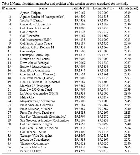
For this study, 30 years (1961–1990) of annual averages from 37 weather stations were used for statistical analysis. Figure 1 shows the locations of the weather stations where the data in this study were gathered. Table I shows the Sistema Meteorológico Nacional name, identification number and detailed position of each station.

Stations were included in the study if they had records of all the following variables: minimum, maximum and mean temperature; precipitation; number of days with appreciable precipitation; days with electrical storms; days with hail; days with fog. Evaporation was not included, as it is not reported by most stations.

The descriptive statistics of the data used in the analysis are shown in Table II. During the recorded period, the mean annual temperature in México City was 15.7 °C with a standard deviation of 2.1 C°. The difference between the minimum and maximum temperatures was 14.5 °C. Average annual precipitation was 827 mm, with a standard deviation of 213. Maximum annual precipitation was 1329 and minimum was 513 mm. The other variables included in the analysis refer to the number of days in a year in which specific phenomena were present, i.e., precipitation, thunderstorms, hail and fog. It is interesting to note the high kurtosis in these variables, indicating the presence of values far from the mean, which confirms the presence of high heterogeneity between some stations and average conditions in the city.

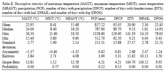
The results of the Jarque–Bera test (Jarque and Bera, 1980) show that the null hypothesis of a normal distribution can be rejected for the majority of the variables (the exceptions being minimum temperature, precipitation, and days with precipitation). This indicates that the variables days with fog, days with hail and days with electrical storms, and minimum and maximum temperature do not follow a normal distribution over México City's territory and that there are stations where these phenomena behave differently. This also could be due to the potential presence of outliers. In addition, it can be observed that most of the variables are not comparable in magnitude, and that variability is much higher in the precipitation variables.

In Table III, a sizeable difference can be observed between the different stations in terms of normal climate variables. In the case of precipitation and temperature variables, zones which are more urbanized tend to show higher temperatures and lower precipitation, while forested zones show the opposite. The common feature of the latter zones is higher elevation. The considerable variability within city is also notable, for an entity which covers a relatively small area. Mean temperature shows a difference of nearly 9°C between station 16 with the lowest temperature and station 8 with the highest mean temperature; the difference between the minimum temperature (station 16) and the maximum temperature (station 8) is equal to 22.5° C. The difference in precipitation between stations 37 and 13 with the lowest and highest precipitation respectively, is 800 mm. At station 9, hardly any electrical storms were recorded, while they occurred on nearly 40% of the days of the year at station 12.

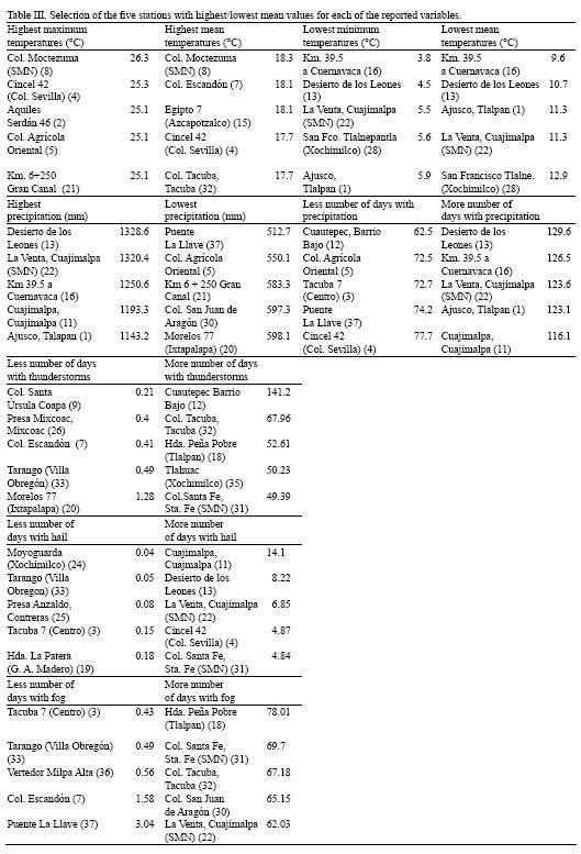
Figure 2 is a star diagram showing all climate variables (scaled) for each of the 37 stations. The stars portray, counterclockwise from right, maximum, minimum, and mean temperatures, precipitation, and days with precipitation, electrical storms, hail and fog. It can be observed that a significant proportion of the stations are dry with high temperatures, little precipitation, and lower electrical activity, hail or fog. Most of these stations are located in the central and northern part of the city at lower elevations (stations 2, 4 and 5, for example). Other stations are wetter with lower temperatures and higher precipitation, corresponding to zones with more vegetative cover and higher elevation (1, 13, 16 and 22, among others), and some stations are notable for their higher proportion of electrical activity, hail and fog (11, 12 and 32).

A clear positive correlation among the temperature variables, and a negative correlation between these and precipitation and the number of precipitation days can be observed in the dispersion matrix (Fig. 3). That is, zones with higher temperatures tend to have less precipitation and fewer days with precipitation. These, as the star diagram shows, generally coincide with more urbanized zones, which may point to the urban heat island effect. The relationship with the number of days with fog, hail or electrical storms is not as clear, and the potential presence of an outlier can be seen in the days with hail and days with electrical storms variables. The graphs of these variables (Fig. 4) show that the atypical observations are from the stations Cuajimalpa (11) and Cuautepec Barrio Bajo (12). The presence of these outlying observations could affect the tests for normality and obscure relationships between the variables. Tests of normality were therefore performed with these observations omitted, and the dispersion and correlation matrices with and without these observations were compared. Neither the tests of normality nor the matrices showed significant changes.

 

3. Multivariate analysis methods

3.1 Cluster analysis

This analysis enables the structure of the "natural" grouping of weather stations to be found (Johnson and Wichern, 2007). The method used in this case was agglomerative hierarchical clustering, which begins by considering each observation as an individual cluster. Then, using some similarity measure (euclidean distance was chosen in this case), and a "linkage" method, first the closest objects are grouped together, then the next closest objects are added, and so on until all the subgroups are grouped into a single cluster. Two linkage methods were used for this analysis, closest neighbor (single linkage) and farthest neighbor (complete linkage). The two methods give different results, the farthest–neighbor method producing clearer and more differentiated clusters in this case.

 

3.2 Principal components

This method seeks to explain the variance–covariance structure of a set of p variables through linear combinations of the variables of the form Y_j= a' _jX, in order to reduce the number of dimensions and enable interpretation of the data.

Principal components are non–correlated linear combinations Y_u Y₂, . . . , Y_P whose variances are as large as possible. The first principal component is the linear combination (a' ₁ X) which maximizes var(a' ₁ X) subject to a' ₁ a₁ = 1. The theorem on maximizing quadratic forms on the unit sphere shows that the maximum is achieved when a₁ = e₁. In other words, this is attained when the vector of constants is the first eigenvector of the variance–covariance (or correlation) matrix and the variance is the first eigenvalue (in order from largest to smallest). The succeeding principal components are those linear combinations (a' _j X) which maximize var(a' _j X) subject to the restriction a' _j , a' _j = 1 and which are not correlated with each other, that is, cov(a' _j X, a' _k X ) = 0 for all j ≠ k. These restrictions are met when the corresponding eigenvectors are chosen to be the respective vectors of constants.

For this study, the matrix of correlations was chosen for calculating the eigenvalues and eigenvectors due to the differences in magnitudes in the variables, and to avoid the variables with the largest magnitudes dominating the principal components.

 

4. Results and discussion

4.1 Cluster analysis

It can be seen in Figure 5 that with a linkage distance of 500, the stations divide into two large groups. In group 1 (left side) the stations join together in a cluster at a much small distance than those in group 2 (right side), indicating that the stations in group 1 are more similar to each other than those in group 2. Upon reducing the distance, we see that the first group to split is group 2 (in which the stations are less similar to each other). At a distance of 300, the cluster we had defined as group 2 divides into two subgroups, and at a distance of 200, group 1 also divides in two, forming a total of four clusters.

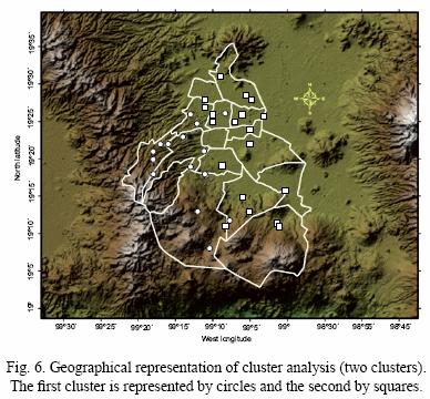
The cluster analysis thus provides evidence that México City contains two large geographic climatic regions defined by topography (Fig. 6). When four clusters are distinguished instead of two, associations between stations in the north and the south are seen to be more longitudinally than latitudinally defined (Fig. 7). The first cluster is located in the eastern part of the city, the lowest region, with suburban characteristics, farmland and lake zones. The second cluster comprises stations located in more urbanized zones and in the lower central fringe. The third contains stations located at piedmont, with urban development, and the fourth cluster is made up of stations located in forested areas at higher elevations.

 

4.2 Principal components

It can be seen in Table IV that the first principal component explains 54.73% of the variability in climate reported by weather stations in México City; the second explains 19.11% (cumulative total 73.84%) and the third 11.23% (cumulative total 85.07%). The scree plot (Fig. 8) shows the values of the eigenvalues and how much each principal component contributes to explaining the variance. According to this figure, the most important principal components are the first two. Nevertheless, although the third eigenvalue is smaller than one, it was decided to include the third component, since its interpretation may contribute important information on climate variability in the city.

According to the absolute values of the elements of the first eigenvector, the most important variables in the first component are mean temperature, maximum temperature, minimum temperature, precipitation, and days with precipitation. It can be seen in Table V that these are also the variables most correlated with the first principal component. It is important to note that the coefficients associated to the temperature variables have negative signs and that those associated to the precipitation variables have positive signs in this component. This means that high values of the first principal component correspond to low temperatures and/or high precipitation. The first component can therefore be interpreted as a measure (index) of how wet or dry the location is. In this respect, Figure 9 shows how the climate of México City increases in moisture from northeast to southwest (cooler temperatures and/or greater precipitation towards the southwest and higher temperatures and/or less precipitation towards the northeast). This figure shows 54.73% of the variability reported by the weather stations. As mentioned above, dryer climates are associated with greater urbanization (heat island effect) and moister climates with regions that have more vegetation and that are located at higher altitudes.

The second principal component explains 19.11% of the variance, and the absolute values of the elements of the second eigenvector show that the most important variables of this component are the number of days with electrical storms and the number of days with fog, which are also the variables most correlated with the second principal component (Table V). In this component, the coefficients associated to both variables have positive signs, meaning that larger values correspond to zones with more electrical activity and/or more fog. Literature on fog dynamics has shown that the UHI produces a significant fog frequency gradient along the urban outskirts (Sachweh and Koepke, 1997). Furthermore, recent studies distinguish the effect of different stages of urban development over the number of days with fog: old urban developments show significant reduction of days with fog, while new urban developments tend to show more days with fog, mainly because in new urbanizations the abundance of hygroscopic aerosols acting as condensation nuclei promote fog formation (Shi et al., 2008). All these factors are present in areas where the index thunderstorms/fog shows high values. The effects of urbanization over thunderstorm occurrence have been shown to be positive and significant and the máximums observed in Figure 10 could be also due to urban piedmont conditions as described in Changon (2001).

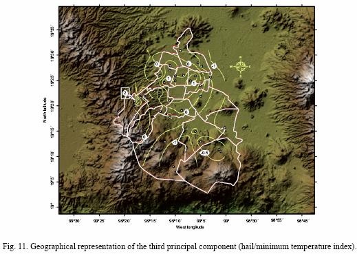
The third component explains 11.24% of the variance. The most important variable in this component, and with which it is most correlated, is the number of days with hail, and to a lesser extent, minimum temperature. The coefficients associated to both variables have positive signs in this component, meaning that higher values correspond to zones with more days with hail and/or zones with higher minimum temperatures. It is interesting to observe (Fig. 11) that the zones with higher values of this component are located in the central–north part of the city, which is the most urbanized. According to urban climatology studies (Jáuregui, 2000), one of the effects of urbanization can be an increase in the number of days with hail and an increase in minimum temperatures (heat island).

To examine the relationship between weather stations, biplots of the principal components were constructed (Figs. 12, 13 and 14). It can be seen in Figure 12 that the majority of stations had similar values, but that a few others had very divergent values. The largest number of stations are concentrated around quadrant III (negative values of the first principal component and negative values of the second component), which represents dryer climates (higher temperatures and/or less precipitation) but with lower electrical activity and/or fog. All of these stations are located in high to medium urbanized, piedmont areas. Quadrant I is notable because it contains only four stations (three in Cuajimalpa [22 and 11] and Santa Fe [31], and one in Tlalpan [18]) and corresponds to humid zones (abundant precipitation and/or low temperatures) and high electrical activity and/or fog, associated with piedmont and medium altitude semi–urban areas. Some studies have suggested that electrical activity could increase in piedmont areas due to the intensification of convective activity produced by the heat island effect of nearby urbanized areas (Changnon, 2001). Quadrant II represents wetter climates with more precipitation and/or lower temperatures and relatively lower electrical activity and/or fog. The quadrant contains a highly concentrated group of stations and three stations (Ajusco [1], Desierto de los Leones [13] and Km. 39.5 on the highway to Cuernavaca [16]) with very high values in the first component. These stations are located in piedmont and high altitude forested zones that are farther from the most highly urbanized area. The remaining observations in this quadrant also have forest remnants or significant vegetation, as is the case of Pedregal (14), Xochimilco (28), Lomas de Chapultepec (34) and Contreras (25) but are closer to the most highly urbanized area. Quadrant IV represents dryer climates with more electrical activity and/or fog, characteristic of more urbanized zones (Jauregui and Romales, 1996; Changnon, 2001; Ntelekos et al. 2007 ). In fact, all stations in this quadrant belong to the group which had been found by means of cluster analysis and which corresponded to the zone characterized by greater urbanization.

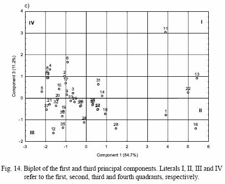
Figure 13 shows the biplot of the second and third principal components. A concentrated group of stations can be observed around negative values of the second component (more electrical storms and/or fog) and a more diffuse group towards positive values of the component. The interpretation of this pattern is not entirely clear, although it does enable outliers to be identified in stations 11 and 31, which have few days with electrical storms and/or fog and more days with hail; and 12, 32 and 18 with few days with electrical storms and/or fog and few days with hail.

The biplot between the first and third principal components (Fig. 14) shows a fairly compact cloud of stations and 5 atypical observations. As in the case of the biplot shown in Figure 12, these five stations are located in semi–urban areas with wetter climates (lower temperatures and/or more precipitation), and are divided between stations with more hail days and/or higher minimum temperatures (Cuajimalpa [11, 22] and Desierto de los Leones [13]) and stations with fewer hail days and/or lower minimum temperatures (Ajusco [1] and Km. 39.5 on the highway to Cuernavaca[16]). Stations in quadrant IV are located in the most highly urbanized area (north–center), describing a dryer climate with higher minimum temperatures and/or more frequent hail. These characteristics have been commonly associated to the urban heat island (Jáuregui and Romales 1996). More humid conditions and with lower minimum temperatures and/or less frequent hail are present at piedmont stations (quadrant II). Quadrant I is composed of stations located at the high altitude western part of México City, showing that conditions are more humid and hail tends to be more frequent. Quadrant III, representing dryer with less frequent hail and/or lower minimum temperatures, corresponds to the eastern, lower altitude part of the city, boarding the most urbanized area.

Although principal components analysis does not require the assumption of normality, if the observations are sampled from multivariate normally distributed populations, inferences can be made and ellipsoids of constant probability density constructed. To test for normality, Q–Q plots were constructed comparing the theoretical quantiles of the normal distribution with the observed quantiles of the principal components. For multivariate normality, all principal components must be normally distributed. For reasons of space, the Q–Q plots are not presented here, but are available upon request. These graphs show that there are significant deviations from the normal distribution in the case of the first and second principal components, while the hypothesis of normality can be accepted for the third component. Three tests of normality (Anderson–Darling, Jarque–Bera and Cramer–von Mises) were performed to confirm these results. As seen in Table VI, the null hypothesis of normality can be rejected for principal components one and two, and accepted for the third. Since multivariate normality is rejected, inferences can not be made on the principal components, nor can confidence intervals for the eigenvalues (explained variance) or ellipsoids of constant probability density be constructed.

 

5. Conclusions

Multivariate statistical methods were used to identify areas with similar climatic conditions and to define climate indices for México City. Results show that the three main climate indexes produced by principal component analysis are able to represent almost all climate conditions of the city, being of particular importance the first principal component which represents about 55% of the climate variability. These three indexes are wetness/dryness, thunderstorms/fog and hail/minimum temperature. The mapping and analysis of these indexes and their biplots provides additional evidence of the effects of the urban heat island in the microclimates of México City, as has been previously shown by Jauregui and Luyando (1998) and Jáuregui (2000). Such studies indicate that urbanization produces a heat island effect that contributes to making climates dryer, with higher temperatures and less precipitation, and may also contribute to increased frequency of hail and fog as well as more intense storms in some areas.

In this paper two climate regions and four climate subregions were identified for México City, suggesting that local climate variability is defined by two main factors which are topography and land use. The four subregions are: low altitude suburban, low altitude highly urbanized, urbanized mountain base, and higher elevation with forests. Results show that while natural factors such as topography play a large role in the variation in meteorological variables, there are also clearly anthropogenic influences that have and continue to modulate spatial climate variability in the city.

The works of Jáuregui (1988, 1991), Martínez–Arroyo and Jáuregui (2000) and Jazcilevich et al. (2000) in México City, and studies in other cities, such as those by the World Meteorological Organization (1996) and Ishi et al. (1991) have found that certain changes in land use can modulate urban microclimates. These provide an opportunity for better urban management, for example introducing green areas and water bodies

The application of simple tools, such as multivariate analysis, to a meteorological network data base enables the various microclimates of the city to be tracked at different times; for example before and after urbanization projects such as construction of arterial roads or large residential zones, or deforestation processes.

 

References

Changnon S. A., 2001. Assessment of historical thunderstorm data for urban effects: the Chicago case. Climatic Change 49, 161–169.        [ Links ]

CONAPO, 2002. Implicaciones demográficas y territoriales de la construcción de un nuevo aeropuerto en la ZMVM. Serie Documentos Técnicos, Consejo Nacional de Población. México.        [ Links ]

Degaetano A. T., 1996. Delineation of mesoscale climate zones in the northeastern United States using a novel approach to cluster analysis. J. Climate 9, 1765–1782.        [ Links ]

Fovell R. G. and M. C. Fovell, 1993. Climate zones of the conterminous United States defined using cluster analysis. J. Climate 6, 2103–2135.        [ Links ]

Ishi A., S. Iwamoto, T. Katayama, T. Hayashi, Y. Shiotzuki, H. Kitayama, J. Tsutsumi and M. Nishida, 1991. A comparison of field surveys on the thermal environment in areas surrounding a large pond: when filled and when drained. Energ. Buildings 15–16, 965–971.        [ Links ]

Jarque C. M. and A. K. Bera, 1980. Efficient tests for normality, homoscedasticity and serial independence of regression residuals. Econ. Lett. 6, 255–259. doi: 10.1016/0165–1765(80)90024–5.        [ Links ]

Jáuregui E., 1988. Local wind an air pollution interaction in the México basin. Atmósfera 1, 131–140.        [ Links ]

Jáuregui E., 1991. Effects of revegetation and new artificial water body on the climate of northeast México City. Energ. Buildings 15–16, 447–455.        [ Links ]

Jáuregui E. and E. Romales (1996). Urban effects on convective precipitation in México city. Atmos. Environ. 30, 3383–3389.        [ Links ]

Jáuregui E. and E. Luyando, 1998. Long–term association between pan evaporation and the urban heat island in México City. Atmósfera 11, 45–60.        [ Links ]

Jáuregui E., 2000. El clima de la ciudad de México. Instituto de Geografía, UNAM– Plaza y Valdés. México, 131 pp.        [ Links ]

Jazcilevich A., V. Fuentes, E. Jáuregui and E. Luna, 2000. Simulated urban climate response to historical land use modification in the basin of México. Climatic Change 44, 515–536.        [ Links ]

Johnson R. A. and D. W. Wichern, 2007. Applied multivariate statistical analysis. 6th Ed., Prentice Hall. New Jersey, 800 pp.        [ Links ]

Jones P. D., P. Y. Groisman, M. Coughlan, N. Plummer, W.–C. Wang and T. R. Karl, 1990. Assessment of urbanization effects in time series of surface air temperature over land. Nature 347, 169–172.        [ Links ]

Martínez–Arroyo A. and E. Jáuregui, 2000. On the environmental role of urban lakes in México City. Urban Ecosystems 4, 145–166.        [ Links ]

Mazzoleni S., A. L. Porto and C. Blasic, 1992. Multivariate analysis of climatic patterns of the Mediterranean basin. Vegetatio 98, 1–12.        [ Links ]

Ntelekos A. A., J. A. Smith and W. F. Krajewski, 2007. Climatological analyses of thunderstorms and flash floods in the Baltimore Metropolitan Region, J. Hydrometeorol. 8, 88–101.        [ Links ]

Oke T. R., 1973. City size and the urban heat island. Atmos. Environ. 7, 769–779.        [ Links ]

Sachweh M. and P. Koepke, 1997. Fog dynamics in an urbanized area. Theor. Appl. Climatol. 58, 87–93.        [ Links ]

Shi C., M. Roth, H. Zhang and L. Zihua, 2008. Impacts of urbanization on long–term fog variation inAnhui Province, China. Atmos. Environ. 42, 8484–8492.        [ Links ]

Tejeda–Martínez A. and E. Jáuregui–Ostos, 2005. Surface energy balance measurements in the México City region: A review. Atmósfera 18, 1–23.        [ Links ]

WMO, 1996. Climate and urban development. World Meteorological Organization, No. 844, Geneva.        [ Links ]