Climate change scenarios of extreme temperatures and atmospheric humidity for México

 

A. TEJEDA–MARTÍNEZ
Grupo de Climatología Aplicada, Departamento de Ciencias Atmósféricas
Universidad Veracruzana, Xalapa, Veracruz, México
Corresponding author; e–mail: atejeda@uv.mx

C. CONDE–ÁLVAREZ
Centro de Ciencias de la Atmósfera, Universidad Nacional Autónoma de México
Circuito Exterior, Ciudad Universitaria, México, D. F., 04510 México

L. E. VALENCIA–TREVISO
Grupo de Climatología Aplicada, Departamento de Ciencias Atmosféricas
Universidad Veracruzana, Xalapa, Veracruz, México

 

Received November 13, 2007; accepted June 3, 2008

 

RESUMEN

En este artículo se presentan escenarios de cambio climático referidos a temperaturas extremas y humedad atmosférica para las décadas de 2020 y 2050. Fueron generados para México a partir de los modelos de circulación general GFDLR30, ECHAM4 y HADCM2. El escenario base corresponde a las normales climatológicas del periodo 1961–1990 para 50 observatorios de superficie. Para la mitad de ellos fue necesario estimar empíricamente la presión atmosférica a partir de la altitud y para la totalidad se obtuvieron modelos estadísticos de los promedios mensuales de temperaturas máxima y mínima así como de humedad atmosférica (relativa y específica). Esos modelos estadísticos, combinados con las salidas de los modelos de circulación general mencionados, produjeron escenarios futuros de medias mensuales de temperaturas extremas y de humedad bajo condiciones de cambio climático. Se mostrarán los resultados para un mes representativo del invierno (enero) y otro del verano (julio).

 

ABSTRACT

The following study explores climatic change scenarios of extreme temperature and atmospheric humidity for the 2020 and 2050 decades. They were created for México through the GFDLR30, ECHAM4 and HadCM2 general circulation models. Base scenario conditions were associated with the normal climatological conditions for the period 1961–1990, with a database of 50 surface observatories. It was necessary to empirically estimate the missing data in approximately half of the pressure measurements. For the period 1961–1990, statistical models of the monthly means of maximum and minimum temperatures and atmospheric humidity (relative and specific) were obtained from the observed data of temperature, solar radiation and precipitation. Based on the simulations of the GFDLR30, ECHAM4 and HADCM2 models, a future scenario of monthly means of maximum and minimum temperatures and humidity in climatic change conditions was created. The results shown are for the representative months of winter (January) and summer (July).

Keywords: Extreme temperatures, atmospheric humidity, climatic change, México.

 

1. Background

Usually, models used to create scenarios of climatic change in México provided only means of solar radiation, precipitation and temperature, and not means of extreme temperatures or atmospheric humidity (Conde et al., 1995), which are the variables that are estimated for México in this study. For that purpose, general circulation models (GCM) are used, which produce more reliable simulations of the present climate than the simple climatic models and are, in some cases, a tool for projecting the climate in the future.

Extreme temperatures and atmospheric humidity are key variables for studies related to biodiversity, human thermal comfort, and in the assessments of impacts of climate variability and change on important sectors, such as agriculture and energy demand.

In the mid 1990's the first regional scenarios of climatic change were produced for the country (Conde et al., 2000; Gay, 2000; Conde et al., 1994). In those studies, scenarios of temperature, precipitation and solar radiation were created for 2 × CO₂ conditions, based on the scenario obtained from the means of the period 1941–1970 for 23 sites in México. Afterwards, Conde et al. (1995) and Magaña et al. (1997) created base scenarios of temperature and precipitation from monthly means of temperature and precipitation during the 1951–1980 period. The Canadian Climate Center (CCC) and Geophysical Fluid Dynamical Laboratory (GFDLR30) models allowed the generation of climate change scenarios using the possible changes in temperature and precipitation for México obtained for 2 × CO₂ atmospheric conditions from the outputs of those models. The results show that the temperature could increase between 1 and 2 °C for the CCC model, whereas for the GFDL–R30 model the changes oscillated between 2 and 3 °C. In general, precipitation slightly decreased for the CCC model, while the GFDLR30 model presented an increase of up to 52% (Conde, 2003).

In this paper the HADCM2 (Mitchell et al., 1999), ECHAM4 (Roeckner et al., 1992) and GFDL30 (Manabe et al., 1991, Delworth et al., 2002) models were applied and a base scenario was generated using 1961–1990 period (SMN, SA).

The typical resolution of the HADCM2 model is approximately 50 km horizontally. It is an atmospheric–terrestrial climatic model of limited area and high resolution. It describes the dynamic flow, the cycle of atmospheric sulfide, clouds and precipitation, radiative processes, terrestrial surface and soil thickness. The HADCM2 model considers the atmospheric conditions under hydrostatic balance; including a complete representation of the Coriolis force. It uses a regular latitude–length grid in the horizontal and hybrid vertical coordinates. It has 19 vertical levels; the lowest at 50 m and the highest at 0.5 hPa employing o coordinates (σ = pressure/surface pressure) for the four lowest levels and pure pressure coordinates for three highest levels. The equations are solved in spherical polar coordinates. The horizontal resolution is 0.44 by 0.44° which provides approximately a minimum resolution of 50 km at the equator. It contains the following physical parameters: cloud cover layer, water content in clouds (liquid and solid phase), convection, radiation scheme that includes the seasonal and diurnal cycles of sunshine, calculating flows of short wave and releases which depend on the temperature, of water vapor, O₃, CO₂, clouds and gases. It calculates the boundary layer and flows in surface, as well as gravity waves in the land–atmosphere interface (Palma et al., 2007).

The ECHAM4 climatic model has been developed by the European Center for Medium Range Weather Forecasting (ECMWF), which is the reason why the first letters of the acronym are EC. The ECHAM4 model is made from a set of physical parameters developed at the University of Hamburg (abbreviation HAM). The parameters allow the model to conduct climatic simulations. In addition, the model is considered to be transformed spectrally with 19 atmospheric levels, a T42 type of special resolution (resolution of approximately 2.8° of latitude/longitude). The ECHAM4 model is capable of reducing radiation errors, however it maintains the temperature and precipitation errors (Palma et al., 2007).

The GFDLR30 model was constructed in 1986 in the United States at the Geophysical Fluid Dynamics Laboratory of Princeton, New Jersey. The R30 designation is because it has a rhomboid type of spectral resolution truncated on the 30 wave number. This model has an R30 horizontal resolution (2.25° latitude by 3.75° longitude), 14 vertical levels and realistic topography, a sensorial sunshine variation, a cloud forecast and a "drained" gravitational wave (Delworth et al., 2002).

 

2. Base scenario data

The base scenario is the 1961–1990 meteorological data of 50 meteorological observatories. Their location is shown in the Appendix. In view that specific humidity is not explicitly available, it was necessary to calculate it based on atmospheric thermodynamics. The mean atmospheric pressure of the station was included only on 16 of the 50 surface meteorological observatories used in this paper. Sunshine data is also incomplete in 10 of the observatories. The details of how the database was completed are explained in the following section.

To obtain the specific humidity, the saturation vapor pressure was calculated with the polynomial expression of Adem (1967). This polynomial is in the fourth degree and can be applied to an interval of temperatures from –10 to 50 °C.

The hypsometric equation (Stull, 2000) could not be used in the 34 observatories without data related to the mean annual atmospheric pressure and to the vertical profiles of virtual temperature. To estimate then the mean annual atmospheric pressure for those observatories, an equation of linear regression was generated from the observatories that did provide the pressure data, and thus Eq. (1) was obtained:

where P is the mean atmospheric pressure (in hPa) and Z is the altitude corresponding to the observatory (in meters). The correlation coefficient between pressure and altitude is 0.99 and the mean standard estimation error of Eq. (1) is 20 hPa.

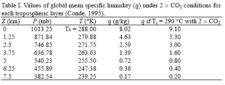
Sunshine hours were estimated in order to calculate relative and specific humidity by means of empirical (statistical) models (see Section 3, Table II). The equation for daily sunshine potential in hours for each site for the 15th day of each month, N₁₅ (Hernández et al., 1991) is calculated with:

with Φ as the latitude and δ₁₅ the solar declination for the 15th day of each month in degrees.

The daily hours of mean monthly sunshine (n) can be obtained from the registers of Campbell–Stokes heliographs, but for sites that do not have heliographic evaluations, Tejeda and Vargas (1996) estimated the monthly mean of cloudiness for each month through the following equation:

Where X₁ is the frequency of cloudy days, when the average of visual observations of the cloud covering is between 6/8 and 8/8; X₂ is the frequency of partially cloudy days (3/8 to 5/8), and X₃ is the frequency of clear days (0 to 2/8).

To calculate the specific humidity, Table II, Tejeda and Vargas (1996) used (29) and (3) to estimate the mean monthly sunshine

 

3. Methods for climatic change scenarios

3.1 Humidity and temperature scenarios

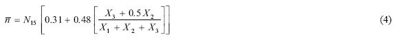
Conde (1995) presented a method for evaluating humidity in the different tropospheric levels on a global scale, via a convective radiative model which considers homogeneous distributions of carbon dioxide at various heights, and obtained the results shown in Table I. However, this information contains, among other forecasts, the generation of atmospheric humidity scenarios at the surface.

For this paper, a direct procedure was applied. For the generation of humidity scenarios for 2020 and 2050 decades surface conditions in México, the mean monthly vapor pressure (e) is estimated according to the monthly mean of minimum temperature (T_mi).

With a₀ = 7.5, a₁ = 8.5 × 10^–2, a₂ = 3.7 × 10^–2, a₃ = –1.7 × 10^–3, a₄ =1.9 × 10^–4, a₅ = –5.0 × 10^–6. The mean standard error is 3.1 hPa and the linear correlation coefficient is 0.91. The relative humidity (RH in decimals) is (Hess, 1959):

Where saturation vapor pressures (in HPa) was calculated through the polynomial of the fourth degree proposed by Adem (1967):

With T (surface mean temperature) in °C and parameter values b₀ = 6.115, b₁ = 0.42915, b₂ = 0.014206, b₃ = 3.046 × 10^–4, b₄ = 3.2 × 10^–6.

From the mean monthly relative humidity, it was estimated the mean monthly values of maximum (RH_m) and minimum (RH_mi) relative humidity. Considering that in the absence of advection, the vapor pressure does not vary between 10 am and 2 pm local time as Geiger (1957) found, the mean minimum relative humidity (representative for 2 pm or 3 pm local time), was calculated through the following equation:

Where RH_mi is the minimum relative humidity, e is the mean monthly vapor pressure and e_sm is the vapor pressure of maximum saturation. The vapor pressure of maximum saturation e_sm was calculated according to the polynomial of Adem (1967) applied to the mean maximum monthly temperature.

The maximum mean monthly relative humidity (RHm) was calculated from the mean monthly relative humidity (RH) as follows:

The increase in the monthly means of minimum and maximum temperatures for the future (2020 and 2050 decades) were obtained from the regional scenarios for México derived from the outputs of the GFDL–R30, ECHAM4 and HADCM2 models applied to México:

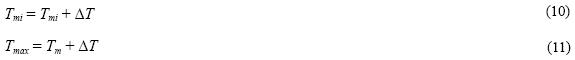
where ΔT is an increase in temperature according to the applied models (Magaña et al., 2000), T_mi is the minimum temperature and T_max is the maximum temperature for the projected scenarios for 2020 and 2050.

Finally, for the estimation of extreme temperatures, Bell et al. (2004) and Phillips and Skindlov (1990) formulas were reviewed. However, to construct the scenarios proposed in this study, a statistical relation was obtained for observed data concerning temperature, radiation and precipitation, with the mean monthly minimum and maximum temperatures and atmospheric humidity (relative and specific). As a result, based on the simulations of the GFDL–R30, ECHAM4 and HADCM2 models, a future scenario was created of mean monthly maximum and minimum temperatures and humidity for 2020 and 2050 scenarios.

For this study, the emission scenarios used were A2 and B2 (Nakicenovic et al., 2000). A2 describes a very heterogeneous world. The underlying theme is self reliance and preservation of local identities. Population growth across regions converge very slowly, which results in continuously increasing population. Economic development is primarily regionally oriented and per capita economic growth and technological change more fragmented and slower than other scenarios. B2 describes a world in which the emphasis is on local solutions to economic, social and environmental sustainability. It is a world with continuously increasing global population, at a rate lower than A2. While the scenario is also oriented towards environmental protection and social equity, it focuses on local and regional levels (IPCC, 2007).

Based on the different statistical relationships previously mentioned, it was possible to create scenarios of extreme temperatures and atmospheric humidity under increased conditions of atmospheric CO₂ for México.

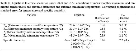
In order to estimate the monthly temperature range (often referred as monthly thermal oscillation), the mean monthly maximum temperature and mean minimum temperature were calculated. The statistical relationships used for every scenario in each variable, and the correlation coefficient and standard error, are shown in Table II. Where Tm₂ is the mean temperature observed in the base scenario (1961–1990 period).

The scenarios presented in the following figures were generated with Eqs. (12) to (15) for temperature and precipitation variables where E are the scenarios created from climatic change, E_i is the base scenario (1961–1990) for minimum and maximum temperature, extreme minimum and extreme maximum temperature and precipitation, ΔT means the mean temperature increase created by the GFDLR30, ECHAM4 and HADCM2 models (Conde, 1995).

Finally, from the increase of specific humidity, the increase in vapor pressure and relative humidity was obtained.

 

4. Results and conclusions

Based on the correlation matrix created from the observed variables, it was determined that there is a statistical relationship among the monthly averages of maximum temperature, minimum temperature and atmospheric humidity based on the monthly averages of temperature, precipitation and sunshine.

There are several basic criteria (IPCC–TGCIA, 2007) to select GCM outputs: vintage (i.e. the most recent results from the GCM); resolution (i.e, some models now have a spatial resolution of 250 km, while their earlier version had 1,000 km); validity (some models simulate the present–day regional climate better than others); and representativeness of results (the chosen models should include a range of values under climate change conditions, i.e. different signs for precipitation). The authors decided that the selected models in this paper covered all the stated criteria.

For the purpose of demonstrating the change in monthly averages of the variables estimated in this study for atmospheric CO₂ duplication, conditions based on the results of the GFDL–R30, ECHAM4 and HADCM2 models, the data obtained from the 50 observatories was divided into 6 zone groups (see Appendix) according to Koppen's climate classification (Garcia, 1988).

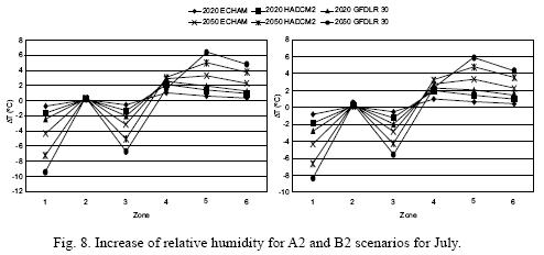
Figures 1 –8 [1, 2, 3, 4, 5, 6, 7 and 8] illustrate the scenarios for January (representative for winter) and July (representative for summer) based on the following variables: mean maximum monthly temperature, mean minimum monthly temperature, extreme maximum monthly temperature, extreme minimum monthly temperature, mean monthly temperature and specific humidity.

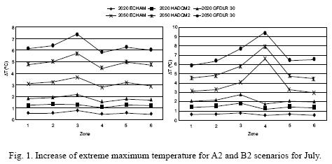
For extreme maximum temperature in July for A2 scenario, all models present a high increase in zone 3, for both horizons of study. For B2 scenario in 2020 zone 3 also has the highest increase in all three models while for 2050 zone 4 was the highest.

For extreme minimum temperature in July, A2 scenario in 2020, it is observed that the temperature difference is around 2 °C in all models. For the 2050 decade there is a bigger difference between 2 and 6 °C in all models. The situation is similar for B2 scenario in 2020, where the difference does not exceed 2 °C for all models, while for 2050 the difference is between 2 and 6 °C approximately. Nevertheless, for both scenarios (A2 and B2), and in both periods of time (2020 and 2050) the highest increase is for zone 3.

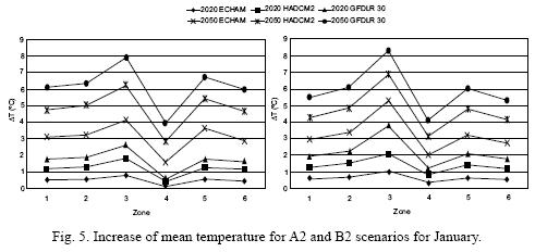
For maximum temperature in January, A2 scenario, 2020, the temperature difference does not exceed 2 °C in all models, whereas for B2 the models present a maximum in zone 3. For 2050 in both models (A2 and B2) the behavior is similar, although for A2 the temperature difference for zone 3 presents a increase of 8 °C, while for B2 it is of approximately 7 °C.

For minimum temperature in January for both scenarios A2 and B2, 2020, the GFDLR3 0 model zone 4 has the highest point with 4 °C. While for 2050, both scenario's tendency is the same, and the GFDL model has an increase of 10 °C in zone 4.

Regarding mean temperature in both scenarios for 2020, for January the maximum point in temperature difference was in zone 3, although for scenario A2 the increase was around 2 °C and for B2 4°C. For the B2 case, there is a strong decay between zones for 3 and 4. For 2050, the temperature difference is of approximately 8 °C in zone 3 for both scenarios, decaying in zone 4 until finding a 4 °C difference.

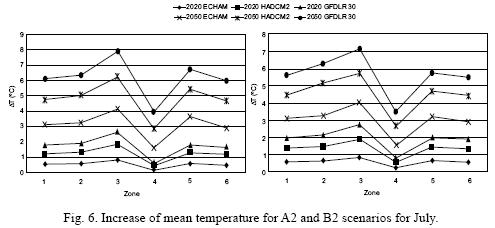
For July, the mean temperature in both scenarios have a similar tendency in all three models for both time periods, although 2020 in A2 has a large temperature difference between zones 3 and 4. For 2050, the maximum point of temperature difference for A2 is 8 °C, while for B2 it is almost the same value, both for zone 3.

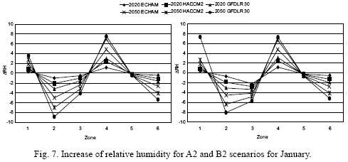
Relative humidity in January in both scenarios for the 2020 period, shows a similar tendency, having its minimum point in zone 2 in all models. For 2050, there is a large difference for the GFDLR30 model in zone 1, being for A2 a difference of 5% and for B2 9%.

Relative humidity in July, both scenarios, also have a similar tendency, being that for the GFDLR30 model zone 1 has the lowest value in both time periods. A strong contrast is found in zone 5 with an approximate 5% value for the GFDLR30 model.

To sum up, it is recommended to carry out additional studies for México with regional models. The problem arising from the use of general circulation models is that many important mountain zones cannot be taken into account given the resolution of the models.

When calculating the means of the possible scenarios for 2020 and 2050 conditions of extreme, and maximum and minimum mean temperatures, we recommend that specific humidity, relative humidity and vulnerability studies of the country should be carried out with respect to its productive activities (i.e. in agricultural and energetic sectors), and also for studies on human thermal comfort for the purpose of developing options for mitigating and adapting to the consequences of climatic change.

 

Acknowledgements

The authors thank Ana María Díaz Díaz and Nury Pavón González for their support to the edition of this text.

 

Appendix

1. Meteorological stations used in this paper and their clustering according to García (1988).

 

References

Adem J., 1967. Parametrization of atmospheric humidity using cloudiness and temperature. Mon. Wea. Rev. 95, 83–88.        [ Links ]

Bell J., L. Sloan and M. Snyder, 2004. Regional changes in extreme climatic events: A future climate scenario. J. Climate 17, 81–87.        [ Links ]

Conde C., 1995. Modelo radiativo–convectivo en la atmósfera. Tesis para obtener el grado de Maestría en Ciencias (Geofísica). Facultad de Ciencias, UNAM, 105 pp.        [ Links ]

Conde C., O. Sánchez and C. Gay, 1994. Escenarios básicos y regionales. In: Estudio de País: México. Primer Taller de Estudio de País: México. México ante el cambio climático. Memorias, Cuernavaca, México, 18 a 22 de abril, 39–43.        [ Links ]

Conde C., O. Sánchez, V. Magaña and C. Gay, 1995. Escenarios climáticos básicos y regionales. In: Estudio de País: México. Segundo Taller de Estudio de País: México. México ante el cambio climático. Memorias, Cuernavaca, México, 8 a 11 de mayo, 101–111.        [ Links ]

Conde C., O. Sánchez and C. Gay, 2000. Escenarios físicos regionales; In: México: Una visión hacia el siglo XXI. El Cambio Climático en México, (V. Magaña Ed.). SEMARNAP, UNAM, USCSP, 1–24.        [ Links ]

Conde C., 2003. Cambio y variabilidad climáticos. Dos estudios de caso en México. Tesis de Doctorado (Ciencias Atmosféricas), Programa del Posgrado en Ciencias de la Tierra, UNAM, 300 pp.        [ Links ]

Delworth T. L., R. J. Stouffer, K. W. Dixon, M. J. Spelman, T. R. Knutson, A. J. Broccoli, P. J. Kushner and R. T. Wetherald, 2002. Review of simulations of climate variability and change with the GFDL R30 coupled climate model. Clim. Dyn. 19, 555–574.        [ Links ]

Fernández A., J. Martínez and P. Hosannilla, 2003. Avances de México en materia de cambio climático 2001–2002, SEMARNAP, INE., México, D. F., 112 pp.        [ Links ]

García E., 1988. Modificaciones al sistema de clasificación climática de Kóppen. Autor Edition. México, D. F., 218 p.        [ Links ]

Gay C. (compilator), (2000). México: Una visión hacia el siglo XXI. El Cambio Climático en México. SEMARNAP, UNAM, USCSP. México, D. F., 220 pp.        [ Links ]

Geiger R., 1957. The climate near the ground. Harvard University Press. Cambridge, UK. 493 pp.        [ Links ]

Hernández, E., A. Tejeda and S. Reyes, 1991. Atlas solar de la República Mexicana. Universidad Veracruzana y Universidad de Colima. México, 155 pp.         [ Links ]

Hess L., 1959. Introduction to Theorical Meteorology. Henry Holt and Co. New York. 39–64 pp.        [ Links ]

IPCC, 2007. Summary for Policymakers. In: Climate change 2007: The physical science basis. Summary for policymakers. Intergovermental Panel on Climate Change. (S. Solomon, D. Qin, M. Manning, Z. Enhen, M. Marquis, K. B. Averyt, M. Tignor and H. L. Miller Eds.). Cambidge University Press, Cambridge, United Kingdom and New York, USA, 18 pp.        [ Links ]

IPCC–TGICA, 2007. General Guidelines on the Use of Scenario Data for Climate Impact and Adaptation Assessment. Version 2. Prepared by T. R. Carter on behalf of the Intergovernmental Panel on Climate Change, Task Group on Data and Scenario Support for Impact and Climate Assessment, 66 pp. http://www.ipcc–data.org/guidelines/TGICA_guidance_sdciaa_v2_final.pdf        [ Links ]

Jáuregui E., A. Ruiz, C. Gay and A. Tejeda, 1995. Una estimación del impacto de la duplicación del CO₂ atmosférico en el bioclima humano de México. In: Estudio de País: México. Segundo Taller de Estudio de País: México. México ante el cambio climático, Memorias, Cuernavaca, México, 8 a 11 de mayo, 219–225.        [ Links ]

Magaña V., 1995. Escenarios Físicos de Cambio Climático. In: Estudio de País: México. Segundo Taller de Estudio de País: México. México ante el cambio climático, Memorias, Cuernavaca, México, 8 a 11 de mayo, 219–225.        [ Links ]

Magaña V., C. Conde, O. Sánchez and C. Gay, 2000. Assessment of current and future regional climate scenarios for México. Clim. Res. 9, 107–114.        [ Links ]

Magaña V., C. Conde, O. Sánchez and C. Gay, 2000. Evaluación de escenarios regionales de clima actual y de cambio climático futuro para México. In: México: Una visión hacia el siglo XXI. El Cambio Climático en México, (V. Magaña Ed.). SEMARNAP, UNAM, USCSP, (C. Gay, Compilador), México, D. F., 15–21.        [ Links ]

Manabe S., R. J. Stouffer, M. J. Spelman and K. Bryan, 1991. Transient response of a coupled ocean–atmosphere model to gradual changes of atmospheric CO₂. Part I: annual– annual–mean response. J. Climate 4, 785–818.        [ Links ]

Manabe, S. and R. Wetherald, 1967. Thermal equilibrium of the atmosphere with a given distribution of relative humidity. Geophysical Fluid Dynamics Laboratory, ESSA, Washington, D. C., J. Atmos. Sci. 24, 241–243.        [ Links ]

Mitchell J. F. B., T. C. Johns, M. Eagles, W. J. Ingram and R. A. Davis, 1999. Towards the construction of climate change scenarios. Clim. Change 41, 547–581.        [ Links ]

IPCC, 2000. Nakicenovic N., J. Alcamo, G. Davis, B. de Vries, J. Fenhann, S. Gaffin, K. Gregory, A. Grübler, T. Y. Jung, T. Kram, E. L. La Rovere, L. Michaelis, S. Mori, T. Morita, W. Pepper, H. Pitcher, L. Price, K. Riahi, A. Roehrl, H.–H. Rogner, A. Sankovski, M. Schlesinger, P. Shukla, S. Smith, R. Swart, S. van Rooijen, N. Victor, Z. Dadi. Special report on emissions scenarios: A special report of working Group III of the Intergovernmental Panel on Climate Change. Cambridge University Press. Cambridge, UK, 599 pp.        [ Links ]

Palma B., C. Conde, R. Morales and G. Colorado, 2007. Escenarios de cambio climático para Veracruz. En: Plan Estatal de Acción Climática del Estado de Veracruz (A. Tejeda–Martínez, coordinador).        [ Links ]

Phillips D. and J. Skindlov, 1990. The Impact of increasing summer mean temperatures on extreme maximum and minimum temperatures in Phoenix, Arizona. J. Climate 3, 1491–1494.        [ Links ]

Roeckner E., K. Arpe, L. Bengtsson, S. Brinkop, L. Dümenil, M. Esch, E. Kirk, F. Lunkeit, M. Ponater, B. Rockel, R. Suasen, U. Schlese, S. Schubert and M. Windelband, 1992. Simulation of the present–day climate with the ECHAM4 model: impact of model physics and resolution Max–Planck Institute for Meteorology, Report No.93, Hamburg, Germany, 171 pp.        [ Links ]

Servicio Meteorológico Nacional s/f. Normales climatológicas periodo 1961–1990.        [ Links ]

Stull R. B., 2000. Meteorology for scientists and engineers. Brooks/Cole Thompson Learning. Pacific Grove, California, USA, 502 pp.        [ Links ]

Tejeda A., 1991. An exponential model of the curve of mean monthly air temperatura, Atmósfera, 4, 139–144.        [ Links ]

Tejeda A. and A. Vargas, 1996. A correlation between visual observations and instrumental records of cloudiness in México, Geofís. Int. 35, 421–424.        [ Links ]

Tejeda A. and D. Rivas, 2001. Un escenario de bioclima humano en ciudades del sur de México, bajo condiciones de 2 × CO₂ atmosférico. El tiempo del clima. Publicaciones de la Asociación Española de Climatología (AEC) Serie A, no. 2., España, 551–562.        [ Links ]

Valencia–Trevizo L. E., 2005. Oscilación térmica y humedad atmosférica en México ante condiciones de duplicación de CO₂ atmosférico. Tesis de Licenciatura en Ciencias Atmosféricas, Universidad Veracruzana, México, 127 pp.        [ Links ]