Analyzing ground ozone formation regimes using a principal axis factoring method: A case study of Kladno (Czech Republic) industrial area

 

L. MALEC, F. SKÁCEL
Department of Gas, Coke and Air Protection, Institute of Chemical Technology in Prague,
Technická 5, 166 28, Prague 6, Czech Republic
Corresponding author: L. Malec; e–mail: Lukas.Malec@vscht.cz

T. FOUSEK
Institute of Public Health, District of Central Czech Republic,
Františka Kloze 2316, 272 01, Kladno, Czech Republic

V. TEKÁC
Department of Gas, Coke and Air Protection, Institute of Chemical Technology in Prague,
Technická 5, 166 28, Prague 6, Czech Republic

P. KRÁL
Institute of Public Health, District of Central Czech Republic,
Františka Kloze 2316, 272 01, Kladno, Czech Republic

 

Received November 5, 2007; accepted January 17, 2008

 

RESUMEN

El ozono troposférico es un contaminante fotoquímico secundario cuyos contenidos están influidos tanto por las razones de emisión de las sustancias contaminantes primarias como por la variabilidad de las condiciones meteorológicas. En este trabajo utilizamos dos métodos estadísticos multivariados para el análisis de la influencia de las condiciones meteorológicas relacionadas con los procesos de transformación de las sustancias contaminantes. Primero, estimamos la variabilidad de la descomposición espacial y temporal de los precursores de ozono mediante el análisis discriminante (DA) en las áreas cercanas a la zona industrial de Kladno (una ciudad de la República Checa). Segundo, interpretamos un conjunto de datos mediante el análisis factorial (FA) para examinar las diferencias entre los procesos de generación de ozono entre las épocas de verano e invierno. Para evitar la dependencia de la temperatura de las variables, así como para describir los procesos troposféricos de lavado de las sustancias contaminantes, utilizamos el contenido de vapor de agua en vez del parámetro de humedad relativa, empleado muy a menudo. De esta manera fuimos capaces de definir con éxito los diferentes procesos de generación de ozono y posteriormente estimarlos junto con la descomposición espacial de sus precursores. La temperatura elevada del aire, la radiación y el bajo contenido de agua están relacionados con los episodios de contaminación en verano, mientras que la radiación y la velocidad del viento resultan ser los parámetros más importantes durante el invierno.

 

ABSTRACT

Tropospheric ozone is a secondary air pollutant, changes in the ambient content of which are affected by both, the emission rates of primary pollutants and the variability of meteorological conditions. In this paper, we use two multivariate statistical methods to analyze the impact of the meteorological conditions associated with pollutant transformation processes. First, we evaluated the variability of the spatial and temporal distribution of ozone precursor parameters by using discriminant analysis (DA) in locations close to the industrial area of Kladno (a city in the Czech Republic). Second, we interpreted the data set by using factor analysis (FA) to examine the differences between ozone formation processes in summer and in winter. To avoid temperature dependency between the variables, as well as to describe tropospheric washout processes, we used water vapour content rather than the more commonly employed relative humidity parameter. In this way, we were able to successfully determine and subsequently evaluate the various processes of ozone formation, together with the distribution of ozone precursors. High air temperature, radiation and low water content relate to summer pollution episodes, while radiation and wind speed prove to be the most important parameters during winter.

Keywords: Air pollution, ozone, discriminant analysis, factor analysis.

 

1. Introduction

The physical and chemical processes of pollutant gases [particularly nitrogen oxides (NO_X) and volatile organic compounds (VOC)] in the troposphere result in the formation of secondary oxidized products. Because many of these processes are regulated by the presence of sunlight, the oxidized products, including oxidants such as O₃, are commonly referred to as 'secondary photochemical pollutants'. The production of high levels of ground ozone is of particular concern, as it is known to act as the primary source of OH (the main atmospheric oxidant) and also as a greenhouse gas. Furthermore tropospheric O₃ has adverse effects on human health, vegetation (e.g. crops) and materials.

It is well–known that ozone content has more than doubled during the past 100 years. Vast regions of the globe are presently experiencing ground ozone levels greater than 40 µL m^–3 (Sitch et al., 2007). These levels, frequently occurring in our study, adversely affect plant production, reduce photosynthetic rates or cause visible leaf injury and plant damage. The temperature–driven increase in biogenic emissions (Vingarzan, 2004) moreover enhances the ozone production throughout the complex chemical cycles.

Road transportation is the dominant source of the O₃ precursors in Europe (39% of total emissions) with energy production, domestic combustion and use of solvents as other key sectors (EEA, 2004). Many recent works (e.g. Meleux et al., 2007; Paoletti and Manning, 2007) show that ozone increases under projected changes in summer European climate and can potentially causes increasing threat to human health and the environment.

In this study, we give only a brief overview of the physical and chemical processes of ozone and other air pollutants, with the reader referred to other publications (Jenkin and Clemitshaw, 2000; Atkinson and Arey, 2003) describing the results of chamber experiments. The principal conditions favourable to ground O₃ formation are known to be solar radiation, high temperatures and stagnant air. In such cases, the photodissociation of NO₂ (UVA wavelength range) can lead to tropospheric O₃ production and the subsequent loss of ozone. These reactions are:

NO₂ + hν O(³P) + NO .............................................(1)

O(³P) + O₂ (+ N₂, O₂) O₃ (+ N₂, O₂)......................... (2)

NO + O₃ NO₂ + O₂..................................................(3)

The occurrence of reactions (1) and (2) is always followed by reaction (3), so that, for a fixed amount of NO2 in sunlit atmosphere, a photostationary state (Leighton, 1961) between the pollutant gases is established on a time scale of ~100 s. However, in the presence of VOC (emitted primarily from various biogenic sources, but also from anthropogenic sources), degradation reactions lead to the formation of intermediate HO2 and RO2 radicals that violate the previous state:

NO + HO₂ (RO₂) NO₂ + OH (RO)................................(4)

Aerosols and clouds occupy a minute fraction of the atmosphere (< 1 mL m^–3 of air in dense clouds), but allow for chemistry that cannot take place in the gas phase, such as ionic and surface reactions (Jacob, 2000). Cloud chemistry is of particular interest in relation to compounds defined by high solubility, and then transformed by rapid hydratation, acid–base dissociation or complexation. Such species can be represented by a wide range of organic compounds (CH₂O, CH₃COOH, HCOOH, etc.), as well as by radicals, H2O2, or reservoir molecules of the nitrogen oxides (HO₂NO₂, HONO, N₂O₅, and particularly HNO₃).

A variety of methods for the statistical modelling of tropospheric O₃ formation have been proposed in the literature over the last decade or so. These can be roughly classified into regression methods, extreme value approaches and space–time models (Thompson et al., 1999). Many of these statistical methodologies apply dimensionality reduction principles (Sirois, 1999), and have been developed to help select a rotation that might produce a solution that is easier to interpret. We decided to use only regression methods to achieve an understanding of the mechanisms underlying pollutant transformations. From the wide range available, we critically selected, and applied, two linear regression methods (multivariate statistical range).

The current state of progress in photochemical behaviour, tropospheric transport processes and the empirical modelling of air pollution transformations has been recently reviewed (Bravo et al., 1996; Spichtinger et al., 1996; Lengyel et al., 2004). In these works, many patterns of factors that cause or hinder O₃ formation regimes were observed. Lengyel et al. (2004) consider the humidity parameter as an outlier. In our study, we contrary suggest the water content to be more reasonable variable in such or similar real situations. The classification and regression tree algorithms represent an alternative approach to methods applied here (Ryan, 1995), primarily from the reason of non–parametricity. On the other hand, interpretation of such methods can result in large extent of consistent over or underpredictions.

Our study use statistical methods reducing dataset dimensionality, revealing temporal and geographical distribution of ground O₃ pollution. Finally, the mutual relationships of all variables considered were carried out.

 

2. Experimental

2.1 Air quality and meteorological data

During the summer of 2006 and the winter of 2007, we conducted two measurement campaigns at five stations situated close to the industrial area of Kladno (50°8'N/14°7'E, 370 m a.s.l.), the largest city in Central Bohemia. The monitoring stations (Fig. 1) were located in north–eastern Kladno (stations abbreviated as DR, DU and UJ), as well as in neighbouring rural zones (stations BU and ST). Choice of this study area was strongly influenced by a number of factors, including the large–scale industrial activity that took place there in the recent past, current industrial activity (metallurgy of iron and steel, engineering, thermal power generation), the proximity of agricultural production to the city, the presence of roads bearing heavy traffic, and its closeness to Prague, the Czech capital.

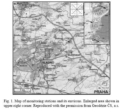
To investigate the geographical distribution of physical and chemical processes in the planetary boundary layer, we used a mobile laboratory (Horiba, Ltd., and ThiesClima – Adolf Thies GmbH & Co. KG) that enabled continuous monitoring of six meteorological and three air pollution parameters. This laboratory was accredited by the Czech Institute for Accreditation, and authorized for the monitoring of air quality by the Czech Ministry of the Environment. Apart from the O₃ parameter, we chose additional variables to represent the atmospheric processes of known pollution episodes: nitrogen oxide and nitrogen dioxide (expressed, as an ozone precursor in the analysis, as the sum of NO_X, and, to quantify mutual relationships, as the ratio of NO₂/NO), air temperature (T), relative humidity, global solar radiation (RAD), atmospheric pressure, wind speed (SPE), and wind direction.

Because of the complex series of reactions driven by air temperature, solar radiation and the variable intensity of emission sources, O₃ formation varies seasonally, daily and even hourly. In order to achieve authentic results, it is necessary to eliminate the effects of such types of periodicity, and a daily cycle was chosen as most representative. To ensure temporal heterogeneity in our investigations, three measurements (all from 3 minute averaging periods), were performed at each station for both summer and winter months. The resulting measurements are numerically identified for each monitoring station.

For all five stations, Figures 2 and 3 present the wind roses for the summer and winter periods, respectively. The density of points, weighted by the wind speed parameter, shows that the majority of the prevailing air masses originated in the north–west and south–west of the region, with some differences occurring between the seasons. These meteorological conditions led us to study the data primarily originating from this mixture of urban, rural and particularly industrial areas.

To achieve a deeper understanding of the heterogeneous processes in the troposphere, all relative humidity values were replaced by water vapour content (identified as H₂O), and such values entered into the analysis. Because systems such as optical hygrometry are susceptible to a high degree of instability under real conditions (WMO, 2006), conversion to volume fraction of water vapour was computed using the Goff–Gratch equation (List, 1984). Based on the experimental data, and taking into account deviations from a perfect gas, the stated range of equation validity is –50 to 102 °C. During measurement, precipitation was controlled (IR–light barrier), and observations relating to rain or snow were deleted.

2.2 Multivariate data analysis

To assess spatial and temporal study of ozone formation processes, the multivariate statistical method of DA was used. This technique enabled us, in the optimum way, to separate out the fifteen measurements (groups) for summer and the fifteen measurements for winter. The daily distribution of NO_X, RAD, T and wind speed parameters revealed the interesting features of local episodes of ground O₃ pollution. However, it was important in our study to be aware of the difference between the discriminant functions and the classification rules that minimize the misclassification rate over allocations.

Once spatial and temporal distribution measurements had been selected using DA, the principal axis factoring solution (FA) was applied to them. Factor analysis seeks to find connections between the variables (O₃, NO₂/NO ratio, H₂O, RAD, T, and SPE) by finding an explanation for the values in the sample correlation matrix. DA and FA have traditionally been described as linear combinations of the original variables and factors, respectively. Some other aspects will be mentioned in the subsection 2.2.1.

All statistical and numerical computations were performed using MATLAB software (The MathWorks, Inc.) and, in particular, its Statistics toolbox. For the needs of this study, the Statistics toolbox environment was modified by standardizing discriminant coefficients, by testing equality of means, and by the development of a factor analysis program (Malec et al., 2007). In the iterative scheme of principal axis factoring, when communality estimates exceed 1 [a situation known as the 'Heywood case' (Heywood, 1931)], iterations continue, and these values are set to 1 for all subsequent iterations.

Various methods of multivariate analysis usually differ with the robustness to the multivariate normality violation of the dataset (Hebák and Hustopecký, 2004). This was the reason to prefer linear technique over the quadratic discriminant function, and to reject the applications of various methods of FA (especially the maximum likelihood method). Our choice partially confirmed the high values of the right–skewness, which ran to the maximum values of: for NO_X 9.705; for NO₂/NO ratio 8.604; and for RAD up to 2.5. Nevertheless, such variables were fourth–root transformed, and, with the exception of the skewness parameter, the resulting effects were examined by means of quantile graphs (unpublished).

2.2.1 Statistical methods

Discriminant analysis is a pattern recognition technique, providing a model determining which variable separate between two or more naturally occurring groups (Krzanowski, 2003; Golub and Van Loan, 1996). The task of this analysis is to find the coefficients of linear combinations (discriminant variables–DV) that maximize the quotient of between–group to within–group variances. The strength of the discriminant function (variance explained) indicates the resulting eigenvalue. The coefficients were then examined to determine which variable contributed strongly to group separation.

Factor analysis is a data reduction method, used to explain correlations among observed variables in terms of unobserved variables called factors. For a numerical realization and under certain conditions, the bilinear model of FA (Rencher, 2002; Golub and Van Loan, 1996) can be expressed:

R = ΓΓ' + ψ, .....................................(5)

where R is the sample correlation matrix, Γ is the matrix of loadings c and ψ is the dispersion matrix of errors. The quantity
h_j² = 1 – ψ_j is defined as the communality of the j–th variable. In other words, the communality of any variable is less than or equal to the reliability of that variable (Harman, 1976). The principal axis factoring estimator c is obtained by maximizing the variance of a factor to all variables using an iterative algorithm. For a clear relation of factors to the original variables, loadings were varimax rotated and the factor score subsequently established.

 

3. Results and discussion

The extent of O₃ and NO_X relations, in which the pairs of correlation/determination coefficients varied from –0.166/0.028 to –0.825/0.681 (summer months), and from 0.085/0.007 to –0.954/0.909 (winter months), confirmed our assumption of VOC–limited conditions (Carslaw and Carslaw, 2001), generally occurring in city centers and polluted regions. The conditions in the latitudes investigated, especially over Europe, generally tend to be varying between the NO_X– and VOC–limited extremes, depending on a given air mass trajectory.

In order to reduce the dimensionality of the complete dataset, DA was used to select six measurements for each period (summer and winter). Then the method of FA was applied to determine the mutual relationships between the variables studied.

3.1 Distribution of ozone precursors

Table I (95th percentile and medians of parameters selected) shows that the summer diurnal phases were of most interest in this study, as this was when O₃ content was at its highest. In some cases the median daily ozone content positively correlates to its elevated levels, while in many cases air temperature strongly correlates with global solar radiation. Moreover high T and high RAD indicate anticyclonic periods in summer, and therefore relate to the high O₃ content. During the winter period, some discrepancies were noticed, and these are discussed below.

As mentioned above, discriminant analysis of the NO_X, RAD, T and wind speed parameters was used to investigate ground O₃ precursors. The DA results (DV coefficients, variance proportion) are shown in Table II. Because of low variances explained by the 4th discriminant variables (0.12% during summer, 0.35% during winter), the corresponding DV were excluded from the analysis. DV1 for the summer months (accounting for 68.53% of the total variance) suggests that parameter T was very important in achieving the maximum differentiation between groups. Similarly, DV2 revealed a high NO_X coefficient value, and DV3 a high SPE coefficient value.

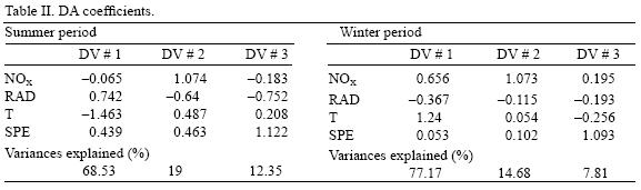
The results for the winter period were much easier to interpret in our study. During the winter months, the mixed effect of RAD (which affected all discriminant variables during the summer period), was heavily suppressed. Nevertheless, DV1 (accounting for 77.17% of the total variance) demonstrated an intermediate connection between the T and NO_X parameters among diverse groups.

In order to test, a priori, the hypothesis of the equality of mean vectors between groups (and thus the usefulness of DA), the Pillai statistic was applied. This statistic, being robust to possible inequalities between sample dispersion matrices (Rencher, 2002), yielded the F–test values of 183.05 (summer) and 420.83 (winter). Consequently, with approximate critical values equal to 1 at all ordinary significance levels, the hypothesis was rejected (Lindley and Scott, 1995) for both seasons.

Figures 4 and 5 display the group centroids of discriminant scores for the summer and winter months, respectively. It should be noted that no causal clustering relationship was significantly observed for either spatial or temporal trends in data. The twelve measurements (summer and winter periods) highlighted in bold were chosen for further analysis. These measurements indicate higher O₃ content during the summer months, and lower O₃ levels during the winter. The winter measurements cover the outliers (particularly BU2 and UJ1), which were clearly responsible for the higher Pillai statistic value (420.83). Owing to such discrepancies, the chosen measurements are considered to be most representative.

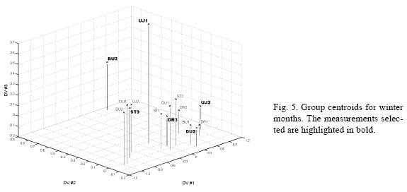
In the summer period, days with O₃–favourable weather patterns were connected with high air temperatures, and with high RAD and low NO_X content (the measurements DU2, UJ2, DU1 and DR1 in Fig. 4). However, in the measurement BU3 high ozone content was only related to NO_X, and here we suspect the occurrence of an atypical situation such as thermal inversion. On the contrary, during the winter, high daily O₃ levels were closely connected to high values of SPE (points clustered on the right in Fig. 5), and to low NO_X content.

3.2 Governing tropospheric processes

To study the variability of ground O₃ formation regimes during the summer and winter months, additional variables such as ozone and H₂O, were entered into FA. Contrary to DA, in FA the parameter NO_X was replaced by the ratio NO₂/NO to describe the photostationary state and the mutual relationships between variables. Two tests, measure of sampling adequacy (Kaiser, 1970), assessing a near–diagonality of matrix R^–1, and the determinant of the sample correlation matrix were performed to reveal the suitability of an iterative approach in the principal axis factoring method. The former test yielded relatively low values, and, therefore, small correlations among the variables. In contrast |R|, while also providing low values [ranging from 5.94 × 10^-4 to 0.0464 (summer) and from 1.95 × 10^-4 to 0.094 (winter)], revealed a high degree of linear dependence among the data.

The number of factors used in our analysis was determined by means of sample correlation matrix eigenvalues greater than 1. For the summer period (at DU1 and DU2), a combination of scree plot and factor model error criteria (introduced in increasing order of significance) was performed. For comparison purposes, prior to interpretation, the whole dataset was analyzed using FA, and the measurements chosen using DA were confirmed as being representative.

The events of the summer period (displayed in Table III) show that positive correlations between the O₃, T and, in some instances, RAD parameters exist, and frequently occur in the 1st factor (F1). Since water vapour absorbs NIR radiation, and because of the scavenging processes of NO₂ reservoir molecules, the above relationship is often negatively counter–correlated to H₂O. In addition, corresponding to reaction (1), the photolysis of NO₂ apparently occurred at BU3 and ST1. O₃ content only relates to SPE at DR2 and ST1, probably as a result of the local cloud dispersion, and the transport of primary pollutants (i.e. NO) from downwind regions.

While the winter period shows many identical relationships to summer, some differences also exist. In particular, the positive correlation of O₃ and RAD prevails above the air temperature parameter, and the NO₂/NO ratio appears to become more important in relation to O₃. Also, the low content of H₂O in ambient air below freezing point (at most 5.4 µL m^–3), reduces its importance and correlation to O₃ levels. At UJ1, we assume the decomposition of NO₂ reservoir molecules (at F2) exceeds the photodissociation of NO₂ with RAD (at F1).

To illustrate the differences between day and night pollutant transformations, the factor scores of BU3 (summer) and UJ1 (winter) are presented in Figures 6 and 7, respectively. These measurements, revealing similar patterns in both seasons, were chosen because they had the lowest |R| values. It is clear that both night observations (covering values < 10th percentile of O₃), and day observations (including values > 90th percentile of O₃) result in two well–resolved clusters that testify to diverse physical and chemical processes.

 

4. Conclusions

Summer and winter air quality and meteorological data, originating from locations close to the Kladno industrial area (a city in the Czech Republic), were used to describe ground O₃ formation. Despite the existence of significant biogenic sources of organic compounds (primarily in the summer months), VOC–limited conditions were found to prevail in this region. Such a situation is very complicated to manage using standard control strategies, so we developed a model that can be used as a guidance tool for the forecasting of O₃ content.

Ordinary statistical methods were not able to accommodate the advection transport of polluted air from upwind regions (Prague agglomeration), together with the slow loss of ozone by deposition. However the two multivariate methods used for data processing in this study were found to offer many important advantages, including:

(a) DA can be used to search for the contributions of ozone precursors to separation measurements, to describe this separation and to reduce the dimension of the dataset.

(b) FA can then be applied to achieve a simpler structure in a set of observed variables, and to determine the physical and chemical processes underlying ground ozone formation.

For comparison purposes, a principal axis factoring program was developed which, in accordance with the methodology used, was not subject to the condition h_j² < 1. In this method, the NO₂/NO ratio was entered according to the mutual relationships of the variables under investigation.

In accordance with differences between the daily measurements, the parameter T at DV1 (accounting for 68.53% of the total variance in summer, and 77.17% in winter) was the most significant of all the precursors considered, followed by NO_X and wind speed. RAD, influential at all DV in the summer months, was less significant during the winter. The high daily mean values of O₃ in the summer period were mostly controlled by high mean values of air temperature and RAD, as well as by low mean values of NO_X. This was not the case in the winter period, where O₃ was mainly dependent on the pollution characteristics of the air masses affecting the Central Bohemian Basin.

Based on the results of our use of FA, a couple of factors were identified for both periods as the main contributors to air pollution in the area studied. In summer, high O₃ content correlated with high T and RAD values, and low H₂O values. In some measurements in situ, photodissociation of NO₂ occurred, while other events were discussed in Section 3.2. In the winter months, high O₃ content was more positively correlated with high RAD (rather than T), and vice versa. The daily measurements for both seasons show that good ventilation conditions (significant SPE values) are positively correlated to O₃ content.

Because of the large increase in temperature and reducing cloudiness projected for global European climate, we expect a higher photochemical production of ozone exceeding internationally accepted environmental criteria.

 

Acknowledgement

This study was supported by a research project of the Czech Ministry of Education pursuant to Contract MSM 6046137304.

 

References

Atkinson R. and J. Arey, 2003. Atmospheric degradation of volatile organic compounds. Chem. Rev. 103, 4605–38.        [ Links ]

Bravo J. L., M. T. Díaz, C. Gay and J. Fajardo, 1996. A short term prediction model for surface ozone at southwest part of México valley. Atmósfera 9, 33–45.        [ Links ]

Carslaw N. and D. Carslaw, 2001. The gas–phase chemistry of urban atmospheres. Surv. Geophys. 22, 31–53.        [ Links ]

EEA, 2004. Environmental signals 2004. European Environment Agency, Kopenhagen, 31pp.        [ Links ]

Golub G. H. and C. F. Van Loan, 1996. Matrix computations. 3rd ed. Johns Hopkins University Press, Baltimore, MA, 728 pp.        [ Links ]

Harman H. H., 1976. Modern factor analysis. 3rd rev. University of Chicago Press, Chicago, 487 pp.        [ Links ]

Hebák P. and J. Hustopecky, 2004. Vícerozmerné statistické metody. Informatorium, Prague, 239 pp.         [ Links ]

Heywood H. B., 1931. On finite sequences of real numbers. Proc. Roy. Soc., A 134, 486–501.        [ Links ]

Jacob D. J., 2000. Heterogeneous chemistry and tropospheric ozone. Atmos. Environ. 34, 2131–59.        [ Links ]

Jenkin M. E. and K. C. Clemitshaw, 2000. Ozone and other secondary photochemical pollutants: Chemical processes governing their formation in the planetary boundary layer. Atmos. Environ. 34, 2499–2527.        [ Links ]

Kaiser H. F., 1970. A second generation Little Jiffy. Psychometrika 35, 401–415.        [ Links ]

Krzanowski W. J., 2003. Principles of multivariate analysis: A user's perspective. Oxford University Press, New York, 585 pp.        [ Links ]

Leighton P. A., 1961. Photochemistry of air pollution. Academic Press, New York, 300 pp.        [ Links ]

Lengyel A., K. Héberger, L. Paksy, O. Bánhidi and R. Rajkó, 2004. Prediction of ozone concentration in ambient air using multivariate methods. Chemosphere 57, 889–896.        [ Links ]

Lindley D. V. and W. F. Scott, 1995. New Cambridge statistical tables. 2nd ed. Cambridge University Press, Cambridge, 96 pp.        [ Links ]

List R. J. (Ed.), 1984. Smithsonian meteorological tables. 6th rev. ed. Smithsonian Institution, Washington, 527 pp.        [ Links ]

Malec L., F. Skácel and A. Trujillo–Ortiz, 2007. FA: Factor analysis by principal axis factoring. URL http://www.mathworks.com/matlabcentral/fileexchange/loadFile.do?objectId=14115. Date of consult: April 3, 2008.        [ Links ]

Meleux F., F. Solmon and F. Giorgi, 2007. Increase in summer European ozone amounts due to climate change. Atmos. Environ. 41, 7577–87.        [ Links ]

Paoletti E. and W. J. Manning, 2007. Toward a biologically significant and usable standard for ozone that will also protect plants. Env. Pollut. 150, 85–95.        [ Links ]

Rencher A. C., 2002. Methods of multivariate analysis. 2nd ed. Wiley, New York, 708 pp.        [ Links ]

Ryan W. F., 1995. Forecasting severe ozone episodes in the Baltimore metropolitan area. Atmos. Environ. 29, 2387–98.        [ Links ]

Sirois A., 1999. Principal component analysis and other dimensionality reduction techniques: A short overview. Atmospheric Environment Service, Quebec, 139 pp.        [ Links ]

Sitch S., P. M. Cox, W. J. Collins and C. Huntingford, 2007. Indirect radiative forcing of climate change through ozone effects on the land–carbon sink. Nature 448, 791–795.        [ Links ]

Spichtinger N., M. Winterhalter and P. Fabian, 1996. Ozone and Grosswetterlagen (general weather situations). Analysis for the Munich metropolitan area. Environ. Sci. Pollut. R. 3, 145–152.        [ Links ]

Thompson M. L., J. Reynolds, L. H. Cox, P. Guttorp and P. D. Sampson, 1999. A review of statistical methods for the meteorological adjustment of tropospheric ozone. National Research Center for Statistics and the Environment, Technical Report Series, Washington, 37 pp.        [ Links ]

Vingarzan R., 2004. A review of surface ozone background levels and trends. Atmos. Environ. 38, 3431–3442.        [ Links ]

WMO, 2006. Guide to meteorological instruments and methods of observation. 7th ed. World Meteorological Organization. No. 8, Geneva, 563 pp.         [ Links ]