Simple air quality model for a plane source

 

S. MONTECINOS
Centro de Estudios Avanzados en Zonas Áridas, Universidad de La Serena, Benavente 980, La Serena, Chile E–mail: sonia.montecinos@ceaza.cl

 

Received July 11, 2006; accepted September 5, 2007

 

RESUMEN

El objetivo de este artículo es mostrar soluciones analíticas simples de la ecuación general de dispersión para una fuente plana homogénea, paralela a la superficie de la tierra. Construimos primero un modelo unidimensional en el cual se supone una mezcla vertical perfecta (PVMM, por sus siglas en inglés). En una segunda etapa, se agrega la difusión vertical al modelo (GM). Ambos modelos predicen que la concentración crece viento abajo y que, debido al flujo de deposición, permanece acotada. Con el objeto de comprobar la validez de los modelos se analiza la distribución espacial de material particulado PMi₀ en la región saturada Temuco–Padre Las Casas, Chile (38.77° S, 72.63° W) y se compara con lo que predicen los modelos.

 

ABSTRACT

The goal of this article is to show simple, analytical solutions of the general dispersion equation for an homogeneous plane source, parallel to the surface of the earth. At a first step, we construct a one–dimensional model, where a perfect vertical mixture is assumed (PVMM). At a second step, vertical diffusion is added to the problem (GM). Both models predict that the concentration increases downwind and, due to deposition, it remains bounded. In order to analyze the validity of the models, the space distribution of paniculate matter PM₁₀ in the saturated zone Temuco–Padre Las Casas, Chile (38.77° S, 72.63° W) is analyzed and compared with the prediction of the models.

Keywords: Air pollution, air quality models, dispersion models, gaussian models.

 

1. Introduction

A dispersion model solves the mass conservation equations of N chemical constituents, given by the following system of differential equations (Seinfeld and Pandis, 1998; Wayne, 1994; Turner, 1994):

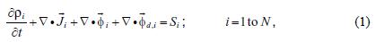
with ρ_i (µg m ^–3) the concentration of the i_th component, (µgm^-2s^-1) the fluxes of advection, diffusion and deposition, respectively. All these variables depend on the space coordinates x, y, z and the time t. The symbol represents the gradient operator defined by:

The advection flux (in the following, we omit sub–index i)

represents the transport of mass by the wind .

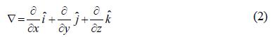
The diffusion or turbulent flux is opposite to the gradient of the concentration p, and is given by:

with K_α = α x, y, z the eddy–diffusion coefficient in α–direction.

The deposition flux can be a very important mechanism to remove pollutants from the atmosphere. Both, particles and gases can be deposited at the earth surface in two ways: dry and wet deposition. The dry deposition can be written as (Finlayson–Pitts and Pitts, 2000)

with the deposition velocity and : the unitary vector perpendicular to the earth's surface, in up direction. Wet deposition is not considered in this work.

Finally, S (µgm^–3s^–1) is the source, including chemical and photochemical reactions. In the following, we assume that the element in study is inert, and therefore the system (1) is reduced to one equation.

To find a solution of equation (1) is in general a complex problem which requires the knowledge of space and time dependence of the wind fields, eddy coefficients, and the characterization of the source. The meteorological variables must be calculated with another meteorological model. Both, dispersion and meteorological models solve the associated equations using numerical methods, which require the appropriated computational infrastructure. Examples of dispersion models are KAMM–DRAIS model (Vogel et al, 1995; Nester and Panitz, 2004) which solves the dynamical equations parallel to the dispersion equation, and the MATCH model, which requires the meteorological fields of an external mesoscale model (Robertson and Langer, 1999).

The formulation of hypothesis makes it possible to find simple analytical or semi–analytical solutions of the original Equation (1). As an example of semi–analytical solution, we mention the works of Moreira et al. (2005, 2006), and Wortmann et al. (2005), which solve the dispersion equation using the generalized integral transform technique (GITT approach). Although the applicability of these solutions is limited, they greatly simplify the analysis of air pollution problems. This kind of air quality models (AQM) in general take the meteorological parameters, which are needed to solve the equations, directly from the observations.

The goal of this article is to develop simple AQM for an homogeneous source, located at a plane parallel to the surface of the earth.

This article is organized as follows: in section 2 we review some AQM found in the literature. We make a brief description of gaussian models for point and linear sources and we make a description of the box model (BM), which corresponds to the most simple solution of equation (6) for a plane source.

In section 3, we construct two solutions of the general equation (6) for aplane source. In section 3.1, we show the model PVMM, where a perfect vertical mixing of the air is assumed. The model describes the downwind evolution of the concentration of an inert pollutant. We use this model to calculate the horizontal scale of influence of the pollutant after it leaves the emission region. In section 3.2, vertical diffusion is added to the problem (model GM). Due to deposition, both models predict a bounded value for the concentration of the pollutant. The bound predicted with PVMM coincides with those calculated with GM at the emission height.

In order to test the validity of the models, the space distribution of particular matter PM₁₀ in the saturated region Temuco–Padre Las Casas, Chile (38.77° S, 72.63° W) is analyzed in section 5. Because the available information is poor, only a qualitative validation is shown. We find that experimental results are in agreement with the prediction of the models.

 

2. Air quality models

In this section we describe known AQM solutions of the general equation (1), which are often used to analyze air pollution problems for simple meteorological conditions. The models assume that the following conditions are satisfied:

• the pollutant is inert,

• both, wind vector u and eddy diffusion coefficients K_α, α= x,y, z, are constant with the space coordinates.

• the system is in quasi–stationary state

• the fluid is incompressible

• the soil is smooth enough to be considered flat. Under these assumptions, equation (1) takes the form:

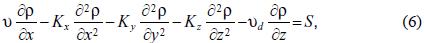
where the coordinate system is chosen in a way that the wind . In the following, we present particular solutions of the above equation, for homogeneous point, linear and plane sources.

2.1 Gaussian models

We consider the case that the emission is continuous, coming from a point source,

where the source is located at the point (0, 0, h), with h the effective height of the source (Hanna et al., 1982). In (7) q (µgs^–1) is the net emission flux, and δ(x) the Dirac distribution (Dirac, 1958; Arfken and Weber, 1971).

If the x–component of the diffusion flux can be neglected in opposite to the advection flux, equation (6)–(7) reduces to:

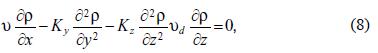
restricted to the border condition (Etling, 2002)

Equation (8)–(9) is known as the Fokker–Planck equation (Gardiner, 2004).

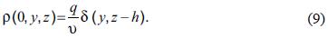
If the deposition flux the solution of (8) is given by (Etling, 2002; Seinfeld and Pandis, 1998; Turner, 1994; Wark et al, 1998)

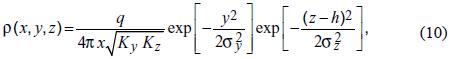
whose profile corresponds to a gaussian curve, with standard deviation

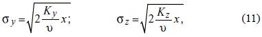
in the y, z direction, respectively. The solution (10)–(l 1) shows, that due to the turbulent fluxes, the plume is widened in the directions perpendicular to the wind, as it moves away from the source.

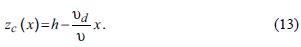
The effect of deposition is to drop the center of the plume to the earth's surface. In fact, it can be shown that, if the solution of (6) is given by:

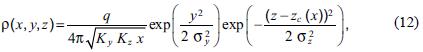
with the center of the plume (Hanna et al., 1982):

This solution reduced to (10) if

The equation (10), or (12), does not consider the effect of the soil on the plume. If the soil completely reflects the plume, we have to impose the following boundary condition (Etling, 2002):

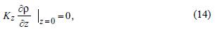
and the solution becomes (Etling, 2002; Turner, 1994; Wark et al, 1998):

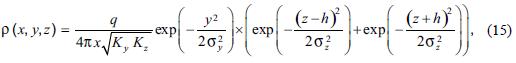
where the second term at the right side is the image flag, which represents the plume produced by a point source located at (0, 0, h).

Now, let us consider the case that the pollutant is produced by a line parallel to the earth's surface. If we choose the y axes parallel to the source, it can be written as:

with Q(µgs^–1) the linear density of emission and h the height of the source.

Due to the linearity of the dispersion equation (8), the concentration at any point (x, y, z) can be written as a superposition of plumes coming from point sources located at (0, y', h) which emits a flux q = Qdy', with y' covering the total emission line.

If the wind is perpendicular to the emission line, and the line is infinite, the solution becomes (Hanna et al., 1982):

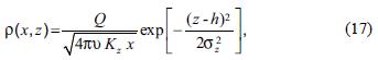
with σ_z given in (11).

It can be shown that (17) satisfies the differential equation (6), for = K_x=K_y = S = 0, restricted to the boundary condition:

Deposition can be taken in to account in a similar way as described above: in (17) replacing with z_c defined in (13). Moreover, if the soil reflects the plume, a plume coming from a line located atz = –h must be added to the solution (17).

2.2 Box model

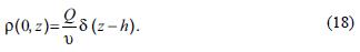
Now we consider the case that the emissions come from a horizontal plane, of the area A =LD. In an appropriate coordinate system, the source can be written as:

with Q (µgm^–2 s^–1) the emission flux. The most simple solution of the general equation (1)–(19), is known as box model (BM) (De Nevers, 1995).

The BM assumes a constant concentration of the pollutant in the box of volume V = LDH. So we have that the diffusion flux and equation (1)–(19) becomes:

with the flux mass and the deposition flux defined in (3) and (5), respectively.

A solution of (20) can be found integrating (20) in the volume V. Using the Stokes theorem (Grant and Phillips, 1991), the integrals can be transformed in surface integrals and equation (20) becomes:

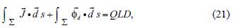
with Σ the surface that evolves the volume V. The above equation corresponds to a mass balance in steady state: the mass that leaves the volume Fby time unit due to advection and deposition, is equal to the mass injected by the source to it.

According to the hypothesis of the model, there exists advection flux only in the lateral sides perpendicular to the wind, and so 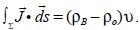with ρ_B the concentration in the volume Fand ρ_o = ρ (x = 0) the background concentration; also the concentration at the beginning of the emission region.

On the other hand, deposition flux exists only at the underlying surface of the cube and so = ρ_B LD. Equation (21) becomes:

If the background concentration ρ_o = 0, we have:

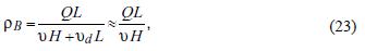
where the term at the right side corresponds to the case:

which is equivalent to neglect deposition flux.

Equation (23) can be used for a first estimation of the concentration of a pollutant, for example, in an urban zone.

We recall that the concentration given in (23) corresponds to a mass balance and so it includes not only the plane source, but also all the sources within the box V.

In the next section, we show that (23) corresponds to the maximum value of the concentration within the box V.

 

3. Air quality model for a plane source

In this section we construct two models to avoid estimating the space distribution of the concentration of a pollutant coming from an homogeneous plane source such as (19). In subsection 3.1, we show the 1–dimensional model PVMM, where a perfect vertical mixture is assumed, and which corresponds to a generalization of the BM. As a particular case, the horizontal scale influence of the pollutant after it leaves the emission region is calculated.

In subsection 3.2, the gaussian model (GM) is constructed. This model corresponds to add vertical diffusion to the problem. As common gaussian models, diffusion parallel to the wind is neglected compared to advection flux.

In both models, PVMM and GM, we assume that the solution does not depend on the horizontal coordinate perpendicular to the wind y.

3.1 One–dimensional model: Perfect vertical mixture (PVMM)

In this section we develop a 1–dimensional model which avoids us to analyze the variation of the concentration in the wind direction x, within the simulation region V=LDH. For the construction of this model, a perfect vertical mixture from the surface of the earth up to the mixing height H is assumed (for definition of mixing height, Holton, 1992).

At a first step, we analyzed the case where diffusion flux is neglected compared to advection flux, and after that, horizontal diffusion is incorporated to the system.

3.1.1 Model without diffusion

We start considering the case K_x = 0, i.e. we suppose that diffusion flux is much smaller than advection flux. The dispersion equation associated to the model is equation (20).

We assume that the concentration p is not constant, but varies downwind. In order to find a solution of equation (20), we divide the total volume V = LDH along x–axis in TVboxes of volume Each box is located at the point x = nΔx.

Now, if Δx is small enough or, equivalent, if TV is large enough, each cube V_n can be consider as a box, where the concentration is constant. So, the results shown in section 2.2 can be applied, if we replace , the size of the volume V_n, and the concentration in volume V_n. Hence, equation (22) is equal to 0:

with ρ₀ = 0

If we divide by Δx and take the limit , the above equation is transformed in the first order, non homogeneous, linear differential equation:

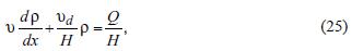
with solution (Amann, 1990):

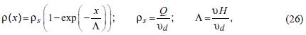
where we have taken the boundary condition ρ(0) = 0.

Equation (26) means that within the emission region the concentration of the pollutant increases downwind, but it remains bounded. We have:

The solution, evaluated for = 5 ms^–1, H=200m, Q = 1µg m^–2s and = 2 cm s^–1, is displayed in Figure 1, curve 1.

We recall that the bound ρ_s does not depend on the meteorological conditions but only on the emission flux Q and the deposition velocity of the pollutant.

The saturation value Q / will be achieved only if the size of the emission plane measured in wind direction Moreover, if , the exponential function can be expanded in Taylor series and we find that the concentration increases linearly downwind:

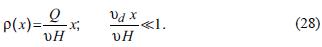
This equation corresponds to neglecting deposition in (25).

The solution (28) is easy to analyze and shows the expected behavior: if the wind intensity increases the concentration of the pollutant decreases, and also decreases if the mixing height goes down.

Now, if we compare the linear solution (28) with the concentration calculated with BM, equation (23), for = 0, we find that:

This result means that BM corresponds to an estimation of the concentration at the end of the emission region, also, to the maximum value of the concentration of the pollutant within the emission region.

3.1.2 Model with diffusion

Equation (26) does not consider the effect of horizontal diffusion on the concentration of the pollutant and so, its validity is subject to the condition:

Now, as we can see in Figure 1, curve 1, the concentration increases very fast near the origin, and so we can expect that diffusion could be important at the beginning of the emission region.

 

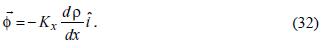
Let us consider the differential equation:

with the turbulent diffusion flux (4), in this case given by

In order to solve equation (31)–(32), we proceed in a similar way as in section 3.1.1: we integrate this equation in the volume and use the Stokes theorem. We obtain

with the concentration and diffusion flux in the cube V_m respectively. Now, we replace (32) in (33), divide by Δx and take the limit So, the equation (33) transforms in the second order, linear, non–homogeneous differential equation:

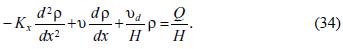
The general solution of the above equation is:

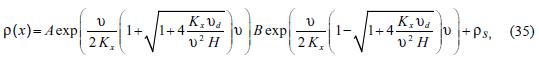
where A and B are arbitrary constants and ρ_s , defined in (26), corresponds to a particular solution of equation (34). We note that the first term at the right side of the above equation diverges if , independent of the value of the diffusion coefficient K_x. So, if we impose that equation (35) must reduce to (26) in the limit it is necessary that the solution remain bounded, and so we have to set A = 0.

If we impose the boundary condition ρ(0) = 0, we obtain:

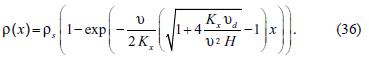
The behavior of the solution is similar to the case K_x = 0: within the emission region the concentration increases downwind until to reach the saturation value Q/v_d . However, due to diffusion, the saturation value is achieved faster. As we can see in Figure 1, curve 1 displays the solution (36) for K_x = 0, also, without diffusion, and curves 2 and 3, the solution for K_x = 3 m² s^–1 and K_x = 3 m² s^–1, respectively.

Comparing both equations (36) and (26), we can conclude that horizontal diffusion can be neglected if:

As an example, if = 5 m s^–1, H = 500 m, K_x = 10 m² s^–1 and if we take = 0.5 cm s^-1, which corresponds to the deposition velocity for fine particles, (Finlayson–Pitts and Pitts, 2000), we find:

In this particular case, horizontal diffusion can be neglected.

We remark that there is a second solution of equation (31) that increases exponentially downwind. Because this solution does not reduce to (26) in the limit we have ignored it. However, if the size of the emission region L is finite, this solution must be, in principle, taken in to account.

 

3.1.3 Scale of influence of the pollutant

In this section we analyze the downwind evolution of the pollutant, once it leaves the emission region. In our analysis we take K_x= 0.

Outside the emission region, the concentration p satisfies the homogeneous differential equation (25), with Q = 0. If we translate the origin of coordinates to the end of the emission region, also, to x = L, the solution is

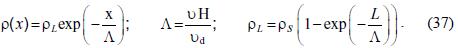
Equation (37) shows that the concentration decreases exponentially downwind. The parameter A represents the horizontal scale factor, which determines the scale of influence of the pollutant. It depends on the meteorological conditions: it increases in conditions of good ventilation and decreases if the mixing height goes down. On the other hand, under similar meteorological conditions, pollutants with a low deposition velocity move farther than those with high ones.

As an example, for 5m s^–1, mixing height H 500 m, deposition velocity _d = 0.5 cm s^–1 (fine particles, size < 2µm, 500 km. Although this value is too large and escapes the validity of the model, this result indicates that particular matter can be transported over long distances, before it deposits. This result is in correspondence to the literature (Gradel and Crutzen, 1992).

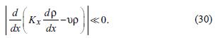
It is important to recall, that the model PVMM corresponds to a mass balance in each volume V_n = ΔxLD, and does not satisfy the original equation (6). In fact, if we put and write equation (31) in cartesian coordinates, and compare the resulting equation with (25), we can conclude that PVMM has implicit the following approximations:

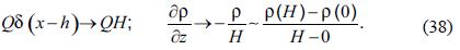
In other words, the source is considered as homogeneous in the volume V = DLH, and the vertical partial derivative of the concentration is approximated by the difference between its value at the earth's surface (z = 0) and at the mixing height z =H, with p (0) = p and p (H) = 0.

3.2 Two–dimensional model: Gaussian model (GM)

In this section we find a solution of the general dispersion equation (6)–(19) which describes the dependence of the concentration in the direction of the wind and the height z. As in the above sections, we assume that the horizontal size of the emission region in the direction perpendicular to the wind is large enough, so that the concentration ρ = ρ (x, z).

In the following, we assume that advection is the predominant flux in x–direction, and that there exists diffusion only in the vertical direction.

3.2.1 Model without deposition

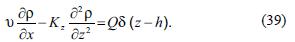
If _d = 0, the (6)–(19) continuity equation becomes:

In order to solve this equation, we apply Fourier transform. We define the function R(x, y), the Fourier transform of the concentration ρ (x, z), as follows (Arfken and Weber, 1971):

where the expression at the right side is the anti–Fourier transform. We proceed as usual: we multiply equation (39) by e^iγz and integrate in z. Hence, we find the following differential equation forR (x,γ):

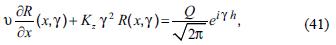
which corresponds to a linear, non–homogeneous, first order ordinary differential equation in the variable x.

The boundary condition needed to solve it, can be obtained from the boundary condition of the original variable p. We have (Arfken and Weber, 1971):

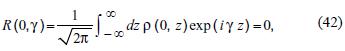
where we have imposed p (0, z) = 0, in a similar way as in PVMM (section 3.1).

It can be directly seen that the solution of (41)–(42) is:

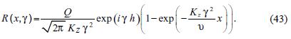
The solution of the original equation (39) can be obtained using (40). We have

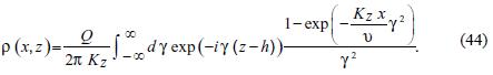
The above solution is symmetric with respect to the emission plane z = h, where it achieves the maximum value. We have:

The integral at the right side can be evaluated directly. We obtain:

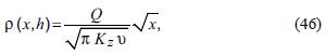
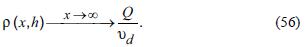
also, at the emission plane the concentration increases downwind proportional to

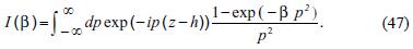
Now, if the integral in (44) does not have an exact primitive. However, a simple algebraic exercise avoids us to transform it in a most simple form.

Let us define the function I(β) as follows

This function satisfies the first order differential equation:

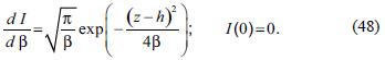
If we integrate this equation, we obtain:

The concentration (44), can be obtained evaluating the above equation in:

We obtain:

which reduces to (46) if z = h.

It is interesting to compare the solution of the GM, equation (50), with the concentration corresponding to an infinite emission line, equation (17)–(11). We can conclude that (50) corresponds to the superposition of flags coming from emission lines perpendicular to the wind, located between the points ζ, = 0 and ζ = x.

Although the integral in (50) has not an exact primitive, it can be solved using simple numerical methods. Figure 2 displays the solution of GM, evaluated for = 5 m s^–1, K_z = 10 m² s^-1, h = 10 m and Q = 1 (µgm² s^-1. For the solution is calculated using the Simpson rule, with the procedure adapted from Numerical Recipes in C (Press et al., 1993). At the left side of the figure, the evolution of the concentration downwind at three different heights is shown: at the emission height z = h, at z = h/2 and at the earth's surface z = 0. At the right side of the figure, the vertical profile of the concentration at x = 10(m) and x = 100(m) is shown. As we have said early, the concentration is symmetric with respect to the emission plane but, opposite to the Gaussian plume, it is not derivable at it.

3.2.2 Model with deposition flux

In order to include deposition in the model, we use equations (50), (12), (13) combined with the superposition principle. So, the solution can be written as the superposition of gaussian plumes coming from infinite emission lines, each one subject to deposition flux We have:

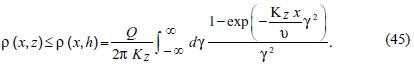
According to the above equation, the solution (51) increases downwind. For z fixed, the concentration remains bounded, as we show in the following.

Let us write (51) in the form:

Because:

we have:

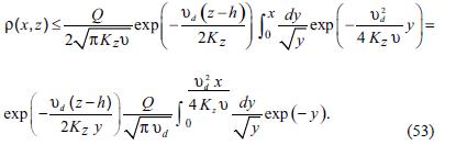
If the integral at the right side converge to:

with the Γ–function defined by Arfken and Weber (1971):

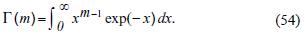
So, we find:

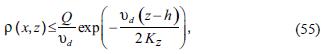
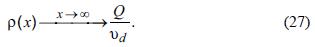
where the equality is valid only at the emission plane, z = h. We have:

We note that the bound at the emission plane coincides with the one obtained with PVMM (see section 3.1, equation (27).

3.2.3 Effect of the earth surface

In a similar way as for a point and a linear sources, described in section 2.1, the effect of the soil can be taken in to account, by adding to the solution (50) a plume coming from an image plane at z= –h.

In the particular case that the emission plane is located at the earth surface z = 0, original and image plumes coincide and the solution is given by:

 

4. Comparison between PVMM and GM

In the above section, we have shown that the asymptotic behavior of models PVMM and GM is similar: both models predict that the concentration of the pollutant increases downwind. Due to deposition, the concentration does not increase indefinitely, but it remains bounded. We found that the upper value of the concentration calculated with PVMM coincides with those calculated with GM at the emission height z = h.

This result is interesting due to the following: in the construction of the models, different hypothesis are assumed and so, both models include different parameters. Besides the common parameter , Q, PVMM depends on the mixing height H and GM on the vertical turbulent coefficient K_z.

Figure 3 displays the downwind behavior of the concentration calculated with PVMM (curve 1), and the one calculated with GM at the emission height z = h, for two different values of the vertical diffusion coefficients, K_z = 5 m² s^–1 (curve 2) and K_z= 10 m² s^–1 (curve 3). The solutions are evaluated for = 5 m s^–1,= 0.05 m s^–1 and Q = 1 µg m^-2 s. For PVMM, the mixing height H=500 m.

According to the early results, the three solutions converge to the saturation value ρ_s = Q l = 20 µgm^–3 in the limit x On the other hand, if K_z = 10 m² s^–1, GM is closer to PVMM than if K_z= 5 m² s^–1.

To find a general relation between H and K_z that minimizes the distance between PVMM and GM at z = h, is a problem that could be studied in a future investigation.

 

5. Validation of the models

The validity of the models presented in this article is restricted to the cases in which the hypothesis of the models are satisfied. So, the PVMM model is valid if the atmospheric conditions imply that a perfect vertical mixture of the pollutant is given. The results of this model could be used in a similar form as the usual BM, we could then omit an estimate of the downwind variation of the concentration of the pollutant.

In this section we analyze the space distribution of particulate matter PM₁₀, also particles < 10 µm in size, measured in two ground stations in Temuco–Padre Las Casas, Chile (38.77° S, 72.63° W, 210,000 inhabitants). Since the available information is not enough to know what model, PVMM or GM, must be applied in this case –the vertical structure of the atmosphere is unknown– and the experimental data measured in two stations are insufficient to analyze the quantitative downwind behavior of the concentration of PM₁₀, the validation shown here is only qualitative. Because both models, PVMM and GM, predicted that the concentration of the pollutant increases downwind, we analyze if this condition is in agreement with the experimental results.

The city of Temuco and neighboring town Padre Las Casas, is threatened by high concentrations of particulate matter PM₁₀ and PM₂₅, especially in autumn and wintertime (from May to October) (Tsapakis et al., 2002). Several studies indicate that wood burning used for house heating, contributes to more than 90% of the emissions of particles. This phenomena has been observed just in 1996 by the Department of Biochemistry and Environment Toxicology of the University of Chile (in Technical Report, CONAMA, 1999). Since November 1998, the Chilean Commission of Environment (CONAMA) has measured the concentration of particles PM₁₀ and the small particles PM₂₅, using Harvard Impactor, with a frequency of 4 days in 6 stations distributed in the city.

Only after June 2000, the Chilean Center of Environment CENMA in cooperation with CONAMA (CENMA–CONAMA, 2001) performs systematic, continuous measurements of PM₁₀ with TEOM equipment (Tapered Element Oscillating Microbalance), in the station Las Encinas (LE). Later, in 2003, a second station of PM₁₀ was installed in the sector of Padre Las Casas (PLC). In both stations, PM₁₀ concentrations and meteorological variables are measured at 10 m height. The location of the two stations is shown in Figure 4.

The results of this campaign are dramatic. In several occasions, concentrations over 800 (µg m^–3) were registered. Only in the period between March and July 2001,17 events in which the concentrations of PM₁₀ exceed the Chilean norm (150 µg m^–3, 24 hours mean value) were detected (CONAMA, 2004). Since these high concentrations have been observed thereafter, in April 2005 CONAMA declared Temuco–Padre Las Casas, as a region over saturated on particulate matter PM₁₀.

Because the principal source of PM₁₀ is the smoke coming from particular houses, the source can, in a first approximation, be considered as an homogeneous plane, and can be written as equation (19). The parameter h represents the mean height of the chimneys.

The analysis shown in this section is based in the CENMA–CONAMA report (CENMA–CONAMA, 2003). We proceed as follows: from the available data (June–September 2003) we choose the data which satisfy, in some approximation, the hypothesis of the models:

• Steady state: we choose episodes where both, PM₁₀ concentration and wind vector, do not present important variations in a period of at least one hour.

• The wind direction θ in both stations is similar. We impose that the maximum deviation Δθ, with respect to the mean value < θ> must be smaller than 15°. This condition is very important because, due to the irregular geometry of the city, small variations in wind direction 0 can introduce important variations in the parameter x, as we can see in Figure 4.

• The chosen episodes have a duration of 2 to 3 hours. In this time interval, we calculate the relevant variables: mean value of wind direction < θ >, mean value of the concentration of particular matter < ρ >, and the distance from the beginning of the city to the station x, measured downwind.

• In order to test the validity of the hypothesis of the model, the maximum deviation of wind direction Δθ, and the mean value of wind < > is evaluated. This last parameter is not used in the analysis.

We recall that in the analyzed cases, the magnitude of the wind in both stations is, in general different. However, this fact is not important: the models shown in section 2 can be generalized for a non–homogeneous wind. The result is similar: the concentration increases downwind.

A description of the analyzed episodes is shown in Table I. The subindex PLC and LE represent the values of the corresponding variables measured in the stations Padre Las Casas and Las Encinas, respectively.

The four episodes shown in Table I are represented in Figure 5. The arrow at the middle of the figure represents the direction of the wind; at the left side, the distance between the monitoring station and the origin of the city x, in arbitrary units, is shown. At the right side of the figure, the variation of the PM₁₀ concentration as function of the distance x is represented. The figure shows that the experimental data are in qualitative good agreement with the models: the concentration increases downwind.

We note that the validation presented in this section is not enough to show the validity of the models presented in this article. Nevertheless, the models correspond to generalization of known analytical, steady state solutions of the general pollutant dispersion equation, and so we can expect that they are valid if the postulated hypotheses are satisfied.

 

6. Summary and conclusions

In this article we show two simple air quality models, also solutions of the general dispersion equation of the concentration of an inert pollutant, for an homogeneous plane source, parallel to the earth's surface. The models could be used to a first analysis of a pollution problem, for example, in a city.

At first we construct the 1–dimensional model PVMM, which assumes a perfect vertical mixture from the surface of the earth aloft to the mixing height. The model corresponds to a generalization of box model and describes the downwind evolution of the concentration of the pollutant.

After that, we show the 2–dimensional model GM, which introduces vertical diffusion to the system. This model generalizes gaussian models to a plane source.

We recall that there exist models in the literature that correspond to numerical solutions of the equation associated to GM, as for example the Airviro system (http://www.indic–airviro.smhi.se), and the ISCST model (http://www.epa.gov/). Opposite to these models, PVMM and GM are essentially analytic and simple to use.

Both models predict that the concentration increases downwind and, due to deposition, it remains bounded. The upper bound of the concentration calculated with PVMM ρ_s = Q /is independent of the meteorological conditions, and coincides with those calculated with GM at the emission height.

The solution calculated with GM shows that the concentration of the pollutant achieves the maximum value at the emission height h.

In order to test the validity of the models, we analyze the downwind variation of the concentration of particular matter PM₁₀ in Temuco–Padre Las Casas (Chile), measured in two ground stations. As predicted by both models, PVMM and GM, we found that the PM₁₀ concentration increases windward.

 

Acknowledgements

This work was supported by project EP120428, Universidad de La Frontera. We thank CONAMA, IX Región, for given experimental data of PM₁₀ concentrations.

 

References

Amann H., 1990. Ordinary differential equations: an introduction to nonlinear equations. Walter de Gruyter, Hawthorne, N. Y, 458 pp.        [ Links ]

Arfken G. B. and H. J. Weber, 1911. Mathematical methods for physicists. Academic Press, Cambridge, University Press, 1200 pp.        [ Links ]

CENMA–CONAMA, 2001. Technical report. A study of the air quality in Chile, Temuco–Padre Las Casas, in order to elaborate a plan of decontamination. Centro Nacional del Medio Ambiente, Comisión Nacional del Medio Ambiente, Chile.        [ Links ]

CENMA–CONAMA, 2003. Technical Report. A Study to the elaboration of an air quality control Programm in Temuco–Padre Las Casas. Centro Nacional del Medio Ambiente, Comisión Nacional del Medio Ambiente, Chile.        [ Links ]

CONAMA, 1999. Technical Report. A study of the Air Quality in Chile, Temuco–Padre Las Casas. Centro Nacional del Medio Ambiente, Comisión Nacional del Medio Ambiente, Chile.        [ Links ]

CONAMA, 2004. Technical Report. Antecedents to declare Temuco–Padre Las Casas as a PM₁₀ saturated zone. Centro Nacional del Medio Ambiente, Comisión Nacional del Medio Ambiente, Chile.        [ Links ]

De Nevers N., 1995. Air pollution control engineering, Mc Graw Hill, New York, 608 pp.        [ Links ]

Dirac P. A. M., 1958. The principles of quantum mechanics, 4th ed. Oxford Sciences Publication, 314 pp.        [ Links ]

Etling D., 2002. Theoretische meteorologie. Eine einfilhrung. 2nd. ed., Springer Verlag, 354 pp.         [ Links ]

Finlayson–Pitts B. and J. Pitts, 2000. Upper and lower atmosphere. London, Academic Press, 969 pp.        [ Links ]

Gardiner C. W., 2004. Handbook for stochastic methods for physics, chemistry antinatural sciences, 3rd ed., Springer Verlag, 415 pp.         [ Links ]

Gradel T. E. and P. J. Crutzen, 1992. Atmospheric change: an earth system perspective. W. H. Freeman, New York, 446 pp.        [ Links ]

Grant I. S. and W. R. Phillips, 1991. Electromagnetism. 2nd. Ed., John Wiley and Sons, 542 pp.        [ Links ]

Hanna S. R., G. A. Briggs and R. P. Hosker, 1982. Handbook on atmospheric diffusion. Technical Information Center, U.S. Departament of Energy, Springfield, VA 22161, 102 pp.        [ Links ]

Holton J. R., 1992. An introduction to dynamic meteorology. 3rd ed., Academic Press, 511 pp.        [ Links ]

Moreira D. M., M. T Vilhena, D. Buske and T Tirabassi, 2006. The GILTT solution of the advection–diffusiom equation for an inhomogeneous and nonstationary PBL. Atmos. Environ. 40, 3186–3194.        [ Links ]

Moreira D. M., M. T. Vilhena, T. Tirabassi, D. Buske and R. Corta, 2005. Near–source atmospheric pollutant dispersion using the new GILTT method. Atmos. Environ. 39, 6289–6294.        [ Links ]

Nester K. and H. J. Panitz, 2004, Evaluation of the chemistry transport model system KAMM/ DRAIS, based on daytime ground–level ozone data. Int. J. Environ. Poll. 22, 87–107.        [ Links ]

Press W. H., S. A. Teukoksky, W. T. Vetterling and B. P. Flannery, 1993. Numerical recipes in C: The art of scientific computing. 2nd., Cambridge University Press, 735 pp.        [ Links ]

Robertson L. and J. Langer, 1999. An eulerian limited area atmospheric transport model, J. App. Meteorol. 38, 190–209.        [ Links ]

Seinfeld J. H. and S. N. Pandis, 1998. Atmospheric chemistry and physics: from air pollution to climate change. John Wiley and Sons, 1145 pp.        [ Links ]

Tsapakis M., E. Lagoudaki, E. G. Stephanou, I. G. Kavouras, P. Koutrakis, P. Oyola P. and P. von Baer, 2002. The composition and sources of PM₂₅ organic aerosol in two urban areas of Chile. Atmos. Environ. 36, 3851–3863.        [ Links ]

Turner D. B., 1994. Workbook of atmospheric dispersion estimates: an introduction to dispersion modeling. Lewis Publishers, 2nd Edition, 635 pp.        [ Links ]

Vogel B., F. Fiedler and H. Vogel, 1995. Influence of topography and biogenic volatile organic compounds emission in the state of Baden–Würtenberg on ozone concentrations during episodes of high temperatures, J Geoph. Res. 11, 22907–22928.        [ Links ]

Wayne R. P., 1994. Chemistry of the atmosphere. University Press, New York, 447 pp.        [ Links ]

Wark K., C. F. Warmer and W. T. Davis, 1998. Air pollution: its origin and control. Harper and Row Publishers, 578 pp.        [ Links ]

Wortmann S., M. T. Vilhena, D. M. Moreira and D. Buske, 2005. A new analytical approach to simulate the pollutant dispersion in the PBL. Atmos. Environ. 39, 2171–2178.        [ Links ]