A numerical investigation of the atmosphere–ocean thermal contrast over the coastal upwelling region of Cabo Frio, Brazil

 

M. DOURADO
Departamento de Meteorologia, Universidade Federal de Pelotas,
Campus Universitário, Caixa Postal 354, 96010–900, Pelotas, RS
Corresponding author; e–mail: marcelo_dourado@ufpel.edu.br

 

A. PEREIRA DE OLIVEIRA
Departamento de Ciências Atmosféricas, Instituto de Astronomia,
Geofísica e Ciências Atmosféricas, Universidade de São Paulo,
Rua do Matão, 1226, 05508–900,

 

Received April 4, 2005; accepted April 24, 2007

 

RESUMEN

En este trabajo se utiliza un modelo atmosférico unidimensional con una cerradura de segundo orden, conectado a un modelo de capa de mezcla oceánica, para investigar las variaciones temporales de intervalo corto de tiempo de las capas límite atmosférica y oceánica en la región de surgencia costera de Cabo Frío, Brasil (23° S, 42°08' W). Se realizaron simulaciones numéricas para evaluar el impacto de los contrastes térmicos entre la atmósfera y el océano sobre la extensión vertical y otras propiedades de estas capas límite. Las simulaciones fueron diseñadas tomando en consideración las observaciones hechas durante la incursión de un frente frío que interrumpió el régimen de surgencia en Cabo Frío en julio de 1992. Las simulaciones han demostrado que, transcurridas 10 horas de mezcla mecánica, debido a una corriente atmosférica constante de 10 m s^–1, aumentó la altura de la capa límite atmosférica en 214 m cuando el contraste térmico inicial es positivo e igual a 2 K (la atmósfera es más caliente que el océano durante la surgencia). Para un contraste térmico inicial negativo de –2 K (la atmósfera es más fría que el océano cuando el régimen de surgencia está alterado), la incipiente convección térmica incrementa la mezcla mecánica incrementando la capa límite atmosférica en 360 m. La evolución vertical de la capa límite atmosférica simulada es consistente con las observaciones en Cabo Frío en régimen de surgencia. Cuando la surgencia no está presente, la altura de la capa límite atmosférica simulada es cerca de la mitad que la observada en Cabo Frío en julio de 1992. Durante el periodo de 10 horas analizando la capa de mezcla oceánica se incrementa en 2 y 5.4 m, respectivamente, para los contrastes térmicos iniciales positivo y negativo de 2 K y –2 K. La extensión vertical de la capa de mezcla oceánica es controlada por la presencia de la convección térmica en la capa límite atmosférica asociada a la ausencia de surgencia y al paso de frentes fríos por Cabo Frío.

 

ABSTRACT

An one–dimensional atmospheric second order closure model, coupled to an oceanic mixed layer model, is used to investigate the short term variation of the atmospheric and oceanic boundary layers in the coastal upwelling area of Cabo Frio, Brazil (23° S, 42°08' W). The numerical simulations were carried out to evaluate the impact caused by the thermal contrast between atmosphere and ocean on the vertical extent and other properties of both atmospheric and oceanic boundary layers. The numerical simulations were designed taking as reference the observations carried out during the passage of a cold front that disrupted the upwelling regime in Cabo Frio in July of 1992. The simulations indicated that in 10 hours the mechanical mixing, sustained by a constant background flow of 10 m s^–1, increases the atmospheric boundary layer in 214 m when the atmosphere is initially 2 K warmer than the ocean (positive thermal contrast observed during upwelling regime). For an atmosphere initially –2 K colder than the ocean (negative thermal contrast observed during passage of the cold front), the incipient thermal convection intensifies the mechanical mixing increasing the vertical extent of the atmospheric boundary layer in 360 m. The vertical evolution of the atmospheric boundary layer is consistent with the observations carried out in Cabo Frío during upwelling condition. When the upwelling is disrupted, the discrepancy between the simulated and observed atmospheric boundary layer heights in Cabo Frío during July of 1992 increases considerably. During the period of 10 hours, the simulated oceanic mixed layer deepens 2 m and 5.4 m for positive and negative thermal contrasts of 2 K and –2 K, respectively. In the latter case, the larger vertical extent of the oceanic mixed layer is due to the presence of thermal convection in the atmospheric boundary layer, which in turn is associated to the absence of upwelling caused by the passage of cold fronts in Cabo Frío.

Keywords: One–dimensional modelling, atmospheric boundary layer, air–sea interaction, upwelling.

 

1. Introduction

The geophysical fluid portion directly affected by the presence of surface is referred to as planetary boundary layer (PBL). The two most notable examples are the atmospheric boundary layer (ABL) and the oceanic boundary layer (OBL) (Large, 1998). Turbulence in these two layers plays a vital role in the interaction between ocean and atmosphere, by controlling exchanges of momentum, heat, and mass in the sea surface. Understanding how ABL and OBL interact is critical for improving numerical weather prediction and climate modeling skills (Weng and Taylor, 2003).

Even though winds are the major source of turbulence in the ABL over the ocean, the intensity of the mechanically produced turbulence can be strongly modulated by the thermal contrast between the atmospheric and oceanic PBL. This thermal contrast, hereafter defined as the temperature of air at 10 m minus the surface temperature of the ocean, can be generated by a variety of atmospheric and oceanographic phenomena. In general, it is stronger near to the continent and looses intensity over open ocean (da Silva et al., 1994). Near continental areas, a stable ABL is frequently found when warm air is advected over cold water (positive thermal contrast) at middle and high latitudes (Smith et al., 1996). Stable ABL are also frequently observed at low latitudes over upwelling regions (Enriquez and Friehe, 1997). Near continental areas, a convective ABL is generated when cold air is advected over warmer water (negative thermal contrast) at all latitudes (Kantha and Clayson, 2000).

The winds are a maj or source of turbulence in the OBL, although at night significant convective mixing takes place. In middle and high latitudes the OBL depth has a strong seasonal cycle due to the recurrent variation of position and intensity of the migratory extra–tropical cyclones. At low latitudes the OBL depth is less variable reflecting mainly the seasonal variations of the trade wind position over the ocean (Kantha and Clayson, 2000). The effects of the thermal contrast in the OBL are less obvious. The production of turbulent kinetic energy due to buoyancy is proportional to the sensible heat flux, which in the OBL depends on the energy budget at the ocean surface.

In the Cabo Frío area (Fig. 1), located at subtropical Atlantic waters in the coast of Brazil (23° S, 42°08' W), the prevailing upwelling regime maintains cold surface water during most of the year, inducing a stable ABL in association to the northeasterly trade wind. Under these undisturbed conditions, the mechanically produced turbulence is attenuated by a positive thermal contrast, limiting the ABL height to a few hundredths of meters. Besides, vertical extent of the OBL is restrained to a few tenths of meters by the upward flow associated to the upwelling dynamics.

During the passage of a cold front, the surface wind direction shifts and, consequently, the upwelling regimen is disrupted. Under this disturbed condition, the surface water warms up and observations indicate that the vertical extents of both ABL and OBL increase (Dourado and Oliveira, 2001). The dynamics of upwelling circulation in the Cabo Frio region has been addressed in the literature (Stech and Lorenzzetti, 1992; Rodrígues and Lorenzzetti, 2001). There are also indications that upwelling intensifies the Seabreeze circulation in the in Cabo Frió region (Franchito et al., 1998). However, the impact caused by short–term variation of the thermal contrast between atmosphere and ocean when the upwelling regime is disrupted has not been investigated. For instance it is not known how much of the short term variation observed in both ABL and OBL structures is related to the modification in the thermal contrast between the atmospheric and oceanic PBL when the upwelling regime was disrupted in Cabo Frio due to the passage of the cold front in July of 1992 (Dourado and Oliveira, 2001).

Planetary boundary layer models can be classified into two categories: slab layer (or single layer) and diffusion (multilevel) models. Slab layer models attempt to reproduce the PBL behavior in a bulk sense (Niiler, 1975; Niiler and Kraus, 1977; Garwood, 1977; Zilitinkevich et al., 1979; Price et al., 1986; Gaspar, 1988). They all assume, a priori, the existence of a well–mixed layer. Observations of isothermal layers have provided the foundation for this approach for ocean, but it is not a universally correct assumption (Large, 1998). In the case of the atmosphere, the slab layer approach can only be justified when the ABL is highly convective (Stull, 1988; Pelly and Belcher, 2001).

In diffusion models the PBL properties are directly parameterized as a function of turbulent mixing. The parameterizations can be drawn from the theoretical and observational knowledge of the atmospheric and oceanic surface layer. It can be also based on modeling of turbulence quantities such as second (Mellor and Yamada, 1982; Gaspar et al., 1990) or third moments (André and Lacarrère, 1985). The major advantage of this more complete approach is that they incorporate more physical information than lower order closure (Kantha and Clayson, 1994; Li et al., 2000; Burchard, 2002; Weng and Taylor, 2003).

In this paper a one–dimensional second–order closure model (Oliveira and Fitzjarrald, 1994) coupled to the mixed layer ocean model (Dourado, 1994) is used to simulate numerically the vertical evolution of the ABL coupled to OBL over the Cabo Frio region. Numerical simulations were carried out to evaluate the relative importance of the thermal contrast on the turbulent mixing intensity in both ABL and OBL. The simulations were set up taking as reference the short–term variation observed in July of 1992, when a cold front system disturbed the upwelling regime in Cabo Frio. In an interval of about 12 hours, it was observed an increase of 1.2 K in the OBL temperature. During this short period, it was observed variation in the ABL height ranging from 200 to 1000 m and in the OBL depth from –13 to –59 m (Dourado and Oliveira, 2001).

Two scenarios were idealized to cover the atmospheric and oceanic changes observed in July of 1992:

• Case A: positive thermal contrast where the ABL is initially set 2° warmer than the OBL to represent an undisturbed condition when the Cabo Frio region is controlled by the upwelling regime (Fig. 2a).

• Case B: negative thermal contrast where the ABL is initially set 2° colder than the OBL to represent a disturbed condition when upwelling regime in Cabo Frio is disrupted by the passage of a cold front (Fig. 2b).

This paper is organized as follows. In section 2, major characteristics of the atmospheric and oceanic models are introduced. The results are shown and discussed in section 3 and, in section 4 these results are summarized.

 

2. Description of the models

In the formulations described below, the vertical coordinate system is oriented upwards for both atmospheric and oceanic models and the origin of the coordinate system are set at the ocean surface. By convention, all atmospheric and oceanic vertical fluxes upward are positive. The over bar and prime indicate mean and fluctuation around the mean, respectively. The atmosphere and ocean systems are considered horizontally homogeneous, therefore all atmospheric and oceanic PBL properties are only function of vertical coordinate z and time t.

 

2.1 Atmospheric second order closure model

The second order closure model used here to simulate the ABL consists of a set of equations formed by the first and second order statistic moments for momentum, virtual potential temperature, and specific humidity (Oliveira and Fitzjarrald, 1994; Dourado, 1994). The statistic moments are obtained by Reynolds averaging the momentum, thermodynamic, and water vapor conservation laws valid for scale of motions in the ABL. The resulting mean motion equations assume the following form:

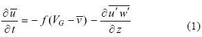
Where and are respectively the zonal and meridional components of the mean wind, U_G and V_G are the zonal and meridional components of the geostrophic wind, f is the Coriolis parameter, is the mean virtual potential temperature, is the mean vertical net radiation flux, is the mean air density and is the mean specific humidity. The covariances between horizontal wind components (respectively zonal and meridional), virtual potential temperature, specific humidity and vertical wind component, respectively , , , and , correspondto the vertical turbulent fluxes of momentum, buoyancy and water vapor in the ABL.

The vertical buoyancy flux is related to vertical flux of sensible heat, , moisture flux, , and mean potential temperature, , by the following expression: = (1 + 0.61) + 0.61 . The vertical component of the mean wind was set equal to zero (Dourado, 1994).

The system of equations above is composed of 8 unknown variables: four first order statistics moments, , four second order statistics moments and 4 equations. This system is completed by including 10 equations for the remaining variances and covariances 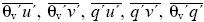. The resulting system is formed by 14 equations and a higher number of unknowns. This closure problem is overcome by specifying all unknown terms as a function of first and second order statistical moments. The closure scheme used here follows Mellor and Yamada (1982). The characteristic length scales used in this closure model are estimated from the modified version of Blackadar expression (Blackadar, 1962) proposed by Mellor and Yamada (1982).

 

2. 2 Oceanic mixed layer model

The mixed layer model used here to simulate the OBL properties is based on an integrated version of the thermodynamic equation and a simplified version of the turbulent kinetic energy (TKE) equation proposed by Zilitinkevich et al. (1979).

This model is based on the following assumptions: (i) The turbulent mixing is strong enough so that upper ocean is characterized by a mixed layer where the temperature does not vary in the vertical direction; (ii) The transition layer between the mixed layer and the stratified non turbulent ocean bellow is much smaller than the mixed layer so that the vertical variation of temperature can be indicated by a temperature jump; (iii) The energy required to sustain turbulent mixing is provided by convergence of the vertical flux of TKE.

Therefore, the ocean surface temperature can be prognosticated by the mixed layer temperature, , given by:

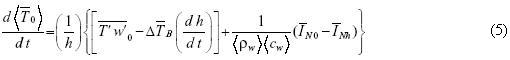
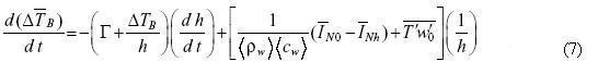
Where h is the depth of the oceanic mixed layer (OML), is the oceanic sensible heat flux at the surface, is the temperature jump at the bottom of the OML, dh/dt is the rate of entrainment of non turbulent water in the OML, and are density and specific heat of water averaged in the OML, and are the net solar radiation fluxes at the ocean surface and at the depth h. At the surface, the net solar radiation flux IN0 is estimated according to Dourado (1994). At depth is evaluated from: = ,exp (γh) where γ = 0.2 m ¹ (Sui et al., 1991).

The mixed layer depth and temperature jump are estimated from:

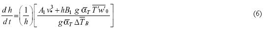
Where g is gravity acceleration (9.81 m s^–2), is thermal expansion factor, Γ is the vertical gradient of temperature in the ocean immediately below the OML, v* is the oceanic friction velocity, B₁ = 0.5 and A1 = 3.4 and (Zilitinkevich et al., 1979).

Equation (6) applies only if there is thermal convection in the OBL ( < 0). When becomes positive the second term in the right side of (6) is set equal to zero.

 

2.3 Boundary and coupling conditions

The upper boundary condition for the ocean and lower boundary condition for the atmosphere are provided by two coupling conditions between ocean and atmosphere. One coupling condition is accomplished by setting the Reynolds stress in the bottom of ABL equal to the Reynolds stress in the top of the OBL. This condition allows one to estimate the oceanic friction velocity in terms of atmospheric friction velocity according to the expression:

In expression (8) u* is the atmospheric friction velocity given by bulk expression: , where is the wind speed at reference level (assumed equal to 10 m) and C_D is the drag coefficient.

Another coupling condition is provided by the energy budget equation at the ocean surface. In this case, the oceanic sensible heat flux at the surface (or at the top of the OBL) is given by:

Where R_N0 is the atmospheric net radiation flux at the surface hereafter indicated by net radiation and evaluated according to Dourado (1994); H₀ and LE₀ are the atmospheric sensible and latent heat fluxes at the surface.

At the surface, the atmospheric sensible heat flux is evaluated from: H₀ = , where is the specific heat of the air at constant pressure (1004 J K^–1 kg^–1) and θ_* is the characteristic temperature scale. In this case θ_* is given by the bulk expression: , where is the potential temperature at reference level, is set equal to the potential temperature at the surface and C_H is the bulk transfer coefficient of sensible heat. The atmospheric pressure at the surface is set equal to 1013 hPa and kept constant during all simulations. Potential temperature is evaluated from the virtual potential temperature and specific humidity using the following relation: =

The latent heat flux at the surface is evaluated from: LE₀ = – , where is the latent heat (2.5 X 10⁵ J kg^–1) and q_* is the characteristic scale of specific humidity. In this case q_* is given by the bulk expression, where is the specific humidity at the reference level, q₁ is set equal to the specific humidity of saturation at the surface temperature and C_E is the bulk transfer coefficient moisture.

The drag coefficient (C_D) and the bulk transfer coefficients of heat (C_H) and moisture (C_E) are estimated in terms of the stability of the surface layer (Dourado, 1994).

 

2.4 Numerical scheme

In the atmosphere, the equations for the mean quantities, like horizontal wind components, virtual potential temperature and specific humidity (1–4) are solved by finite difference techniques using a numerical scheme forward in time and centered in space. The equations for variances and covariances are solved using an implicit numerical scheme (Dourado, 1994).

The mean and second statistic moment variables are allocated on a staggered grid, where the vertical grid space varies logarithmically in the surface layer and linearly in the upper levels. It was used a grid with 81 points evenly distributed over a transformed vertical domain of 13.54 m (1000 m in the z–domain). In the z coordinate, the resulting vertical resolution varies from 4.1 m, near the surface, to 15.41 m at the upper domain boundary.

The thermal effects due to the interactions between radiation and atmosphere are neglected in (3). These interactions were taken into consideration only in the heat budget equations, (5), (6), (7) and (9) at the surface and within the ocean.

In the ocean the equations for OML temperature, temperature jump, and OML depth (5–7) are solved using a finite difference scheme forward in time. The numerical schemes used in the atmospheric and oceanic boundary layers are kept stable for a time step equal to 5 seconds.

 

2.5 Initial conditions

The simulation is carried out using as initial condition the average vertical profiles of virtual potential temperature and specific humidity observed during the observational campaign of 1992 in Cabo Frio (Dourado and Oliveira, 2001).

Since there was no wind measurements during this campaign the initial condition for wind was obtained from the available synoptic charts (Dourado, 1994). Above 200 m, the flow was considered in geostrophic equilibrium, with a geostrophic wind constant in the vertical and from east (Fig. 3, Table I). Below 200 m the wind was assumed to vary logarithmically with height.

The initial profiles of the variances and covariances are obtained by running the model during one hour and keeping the mean quantities constant. During this initialization procedure the OML model was not run.

Table I shows the initial values of thermal contrast, difference between the potential temperature at 10 m and potential temperature at the ocean surface , geostrophic wind component values (U_G and V_G) and oceanic mixed layer model parameters used in the simulations. The vertical gradient of temperature in the ocean beneath the mixed layer ( Γ ) was also kept constant during the simulation.

 

3. Results and discussion

In this section, the results of the numerical simulation using a second order closure model coupled to an oceanic mixed layer model are presented. To obtain these results the model was run to simulate the time evolution of the atmospheric and oceanic PBL for 10 hours, beginning at 9 LT on year day 189 of 1992. This year day correspond to July 7, 1992, when the cold front penetrated in Cabo Frio area.

 

3.1 Mean structure of the ABL

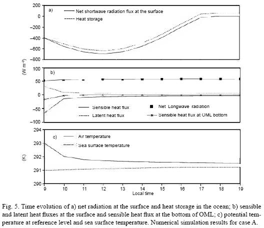
The results for the case A are shown in figures 4 and 5. The formation of an ABL with the top around 414 m is observed at the end of the period of integration, indicating that the ABL has increased about 214 m during 10 hours. The vertical evolution of the ABL can be identified visually by following the virtual potential temperature contour lines in the region near to the surface (contour line 293 K in Fig. 4a). The cooling near the surface is due to the divergence of sensible heat flux in the ABL (continuous line in Fig. 5b).

The time evolution of specific humidity shows an inverse pattern near to the surface, where an initially positive gradient of specific humidity increases slightly with time. This incipient increase in the specific humidity is due to the vertical convergence of moisture flux in the ABL. The moisture flux is indicated by a positive latent heat flux at the surface (dashed line in Fig. 5b).

In case A the ABL vertical evolution is exclusively sustained by the mechanical turbulent mixing (Figs. 4c, d). In this case, the mechanical production of TKE is strong enough to compensate the loss due to the thermal stratification and to the molecular dissipation. The intensification of the vertical wind shear is associated to the formation of a low level maximum and contributes to increase the vertical extent of the ABL (Fig. 4d). This low level maximum occurs mainly in the meridional component reaching about 3 m s^–1 around 150 m at the end of the simulation. The low level maximum is a direct consequence of initial imbalance between the PBL mean flow and the geostrophic wind.

The surface net radiation and oceanic heat storage, defined as + I_N0, show a similar time evolution for case A (Fig. 5a). Their time evolution indicates that the input of energy in the ocean is mainly due to the incoming solar radiation. The radiation cooling of the surface removes energy from the ocean during the transition between day and night, and at nighttime. Despite the large amount of available energy, the amplitudes of the sensible and latent heat fluxes are small in this case (Fig. 5b).

In the case A, during a period of 10 hours, the sensible heat flux varies from –70 to about –5 W m^–2, while the latent heat flux varies from 25 to about 5 W m^–2. The thermal stratification regulates the moisture flux towards the atmosphere, inhibiting the vertical transport of moisture from the surface. The reduction in the amplitudes of the turbulent fluxes of sensible and latent heat is a direct consequence of a diminution in the thermal contrast between atmosphere and ocean (Fig. 5c).

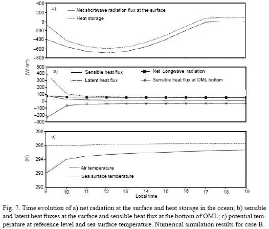
The results for the case B are shown in figures 6 and 7. The ABL top reaches around 560 m at the end of the period of integration indicating that the ABL has increased about 360 m during 10 hours. The vertical evolution of the virtual potential temperature is characteristic of an atmospheric mixing layer (Fig. 6a). In this case, the progressive warming of the atmosphere is consequence of the vertical convergence of sensible heat flux in the ABL, which is a maximum positive at the surface (continuous line in Fig. 7b). The time evolution of the simulated ABL shows a significant increase in the magnitude of the specific humidity in the lower levels (Fig. 6b). This strong input of moisture is due to the intense vertical convergence of moisture flux in the ABL. The moisture flux is also indicated by a positive latent heat flux at the surface (dashed line in Fig. 7b).

In comparison with the case A (Figs. 4c, d), the horizontal wind components in case B had a similar evolution (Figs. 6c, d). In case B, the PBL vertical extent is greater and the area with positive meridional component is larger than in case A. As consequence of a deeper ABL, the amplitude of low level maximum in the meridional component is smaller.

The diurnal evolution of the surface net radiation in case B is very similar to case A (Fig. 7a) but, on the other hand, the ocean stores much less energy in case B. This difference is basically due to the fact that a significantly larger portion of the available energy is transferred to the atmosphere in the form of sensible and latent heat fluxes in case B (Fig. 7b). In this case the sensible heat flux varied from 75 to about 5 Wm^–2, while the latent heat flux varied from 370 to about 50 Wm^–2. The larger amplitude of the latent heat flux is a direct consequence of the presence of relative colder atmosphere over a warmer ocean.

The negative temperature contrast induces thermal convection intensifying the turbulence in the ABL. A progressive reduction in the amplitude is a consequence of the decrease in the thermal contrast between atmosphere and ocean (Fig. 7c). It is interesting to observe that the amplitude of the thermal contrast between atmosphere and ocean in both cases have the same amplitude but different sign (Figs. 5c and 7c). The amplitude and sign of the sensible, latent and radiation fluxes (not shown here) are in good agreement with the observations carried out over the Pacific at equivalent latitude (Godfrey et al., 1991).

The ABL height (Z_i), evaluated as the level where the TKE is equal to 5% of its value of the surface (Stull, 1988), is shown in Figure 8 for cases A and B. The ABL is higher in the case B due to the contribution of thermal production of TKE (reaching about 560 m). These results are in agreement with the observations carried out in Cabo Frio during the period of upwelling (Dourado and Oliveira, 2001). They also agree with the average value of 500 m obtained by Fitzjarrald and Garstang (1981) for the ABL height over the Atlantic during the GATE.

However, the observations in July of 1992 indicated that after the cold front passage the PBL height in Cabo Frio reached 1000 m (Dourado and Oliveira, 2001), almost twice the simulated value in case B. This factor of two between observed and simulated ABL heights is because the mechanical and the thermal productions of TKE are not strong enough in the scenarios given by case A and B. For instance, horizontal advection of cold air behind the cold front would keep the negative thermal contrast between atmosphere and ocean, or even increase it. This effect, not included in our simulations, can intensify the sensible heat flux at the surface (Austin and Lentz, 1999) and consequently the thermal production of TKE and the depth of the ABL.

The drop in the ABL height in the first hour of simulation indicates that although the turbulent field was initially adjusted to the mean field in the atmospheric PBL (section 2.5), the resulting atmospheric PBL was not in equilibrium with the oceanic PBL at beginning of the simulation.

 

3.2 Turbulence structure of the ABL

Figure 9 shows the normalized profiles of turbulent vertical fluxes of sensible heat, latent heat and horizontal wind components for case A and B obtained after 3 hours of numerical simulation, i.e., at 12 LT. The values of u_*, q_*, q_* and Z_i used in the normalization are given in Table II.

The turbulent fluxes of sensible and latent heat decrease linearly with height for case B due to the presence of thermally induced turbulent mixing (Figs. 9a, b). The deviation from linearity observed in the case A for sensible heat flux is consistent with the behavior of stable ABL over continental areas (Sorbjan, 1987).

The normalized vertical profiles of turbulent fluxes of horizontal momentum converge to the same pattern in both cases (Figs. 9c,d). Their vertical variation indicate the expected transfer of momentum from the atmosphere to the surface, with a positive associated with a negative, and with a negative near the surface and positive around z/Z_i = 0.45 associated with positive v near the surface. This local maximum coincides with the upper boundary core of positive values in the meridional wind component. The position of = 0 coincides with the position of the low level maximum wind.

The vertical distribution of virtual potential temperature and specific humidity variances show maximum at the surface only in case B (Fig. 10). This occurs because under convective conditions the largest vertical gradients of virtual potential temperature and specific humidity are located near to the surface (Fig. 6). In the case A, the maximum occurs above the surface layer (continuous line in Figs. 10a, b).

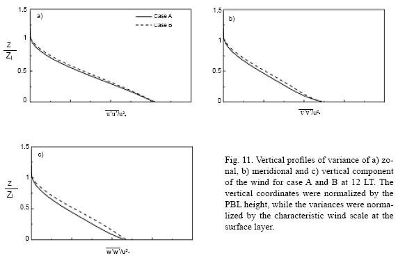
The vertical distributions of variance indicate a maximum at the surface for all three components of the wind in both cases (Fig. 11). This also occurs because the largest vertical gradients of the horizontal wind speed components are located near to the surface. At the surface reached about 3.2 of u²_* while and reached respectively 2.4 and 2.2 of u²_*.. They decrease linearly and coincide in both cases. This behavior is consistent with observations carried out over land (Sorbjan, 1987). These results were expected because the model used here considered the surface of the ocean as aerodynamically rigid. Besides the budget of TKE and other properties have to satisfy the level 2 approximation used as lower boundary conditions (Mellor and Yamada, 1982). In reality, over the ocean surface waves interact with the ABL in such way that the budget of TKE is strongly affected by pressure transport and the vertical distribution of variances of the wind components could be quite different from the ones observed over land (Sjöblom and Smedam, 2003).

3.3 The oceanic mixed layer

The time evolution of simulated OML temperature indicates a maximum variation of 0.22 K in case A and 0.17 K in case B (Fig. 12). Even though they are consistent with the values obtained by LeMone (1980), during phase III of GATE, these variations are about one order of magnitude smaller than the observed variation OML temperature (1.2 °C) during the campaign in 1992 (Dourado and Oliveira, 2001).

The time evolution of the heat storage in the ocean indicated a significant input of energy during most of the period of simulation for both cases (Figs. 5a and 7a). During daytime, this input of energy is responsible for the observed increase in the simulated OML temperature (Fig. 12). Around sunset (17–18 LT), the heat storage becomes positive and the sea surface temperature decreases with time.

The OML depth evolution is indicated in Figure 13. After 10 hours of simulations the OML deepened about 2 m in case A and 5.4 m in case B. These values are very small compared to the 46 m observed in Cabo Frio during equivalent period (Dourado and Oliveira, 2001).

The small OML depths are due to the lack of buoyancy production of TKE in the OML in both cases simulated here. In both simulations, the sensible heat flux at the top of the OML remains positive (Figs. 5b and 7b).

Another factor that reduced the rate of entrainment in these simulations are the values for temperature jump (in the base of the OML) and for the thermal stratification of the ocean below the OML. Even though the used values were obtained from the available observation (Table I) they seem to be large enough to restrain the vertical evolution of the OML (Dourado and Oliveira, 2001).

The intensity of the atmospheric turbulence has a strong impact on the deepening of the OML (Fig. 13). The OML depth is larger in case B because the atmospheric turbulence is stronger. This result corroborate the fact that OBL evolution in Cabo Frio is strongly regulated by the upwelling dynamics (Stech and Lorenzzetti, 1992; Rodrígues and Lorenzzetti, 2001). These dynamic effects that increase the vertical extent of the OBL when the upwelling regime is disrupted, and substituted by downwelling regime, were not included in the simulations carried out in this work.

It was observed during the passage of a cold front in the area of Cabo Frio a large reduction in the incoming solar radiation at the surface due to clouds (Dourado and Oliveira, 2001). Reduction in the incoming solar radiation at the surface would reduce the negative buoyancy flux at the ocean surface (9), reducing the dissipation of TKE in the OBL and intensifying the turbulent mixing in the OML. This effect could not be reproduced here because no cloud effect on solar radiation was included in the simulation carried out.

Another important mechanism that intensifies the turbulence in the OML and was not included in the model used here is the turbulent convective mixing in the bottom boundary layer (Moum et al., 2004). The convective mixing at the bottom boundary layer is particularly important during the coastal downwelling regime as observed in Cabo Frio after the passage of a cold front (Dourado and Oliveira, 2001).

 

4. Conclusions

The aim of this study was to apply a one–dimensional second order closure model coupled to an oceanic mixed layer model to investigate the role played by the thermal contrast between atmosphere and ocean on the atmospheric and oceanic PBL properties over the coastal upwelling region of Cabo Frio, Brazil.

Two scenarios were designed to cover the range of atmospheric and oceanic conditions observed in Cabo Frio in July of 1992. In case A, a positive thermal contrast was imposed to the atmospheric and oceanic PBL, where the ABL was initially set 2 degrees warmer than the OBL. Case A represents the condition observed when the upwelling regime is prevailing in Cabo Frio. In case B, a negative thermal contrast was imposed to the atmospheric and oceanic PBL, where the ABL was initially set 2 degrees colder than the OBL. Case B represents a disturbed condition observed when the upwelling regime in Cabo Frio is disrupted.

The results indicate that the height of atmospheric PBL reached, after 10 hours of simulation, 414 m for case A and 560 m for case B. The result for case A (upwelling condition) is comparable with the ABL height values observed in Cabo Frio before the passage of the cold front in 1992. However, after the passage, the cold front in Cabo Frio, of the observations indicated that the PBL height reached about 1000 m (Dourado and Oliveira, 2001), almost twice the simulated PBL height value for equivalent condition (Case B).

The vertical profiles of variances and covariances of virtual potential temperature, specific humidity, zonal, meridional and vertical wind components are similar to cases of the predominance of mechanical forcing over land. The variances of virtual potential temperature and specific humidity show an important dependence on the thermal contrast

The numerical simulations indicate that the OBL deepens, after 10 hours, about 2 m in case A and 5.4 m in case B. The simulated evolution of the OML depth in both cases are small compared to the deepening of 46 m observed in Cabo Frio during an equivalent period of time (about 12 hours). The simulated OML temperature reached 0.22 K in case A and 0.17 K in case B, about one order of magnitude smaller than the variation of the OML temperature observed in Cabo Frio (1.2 K)

These results indicate that the thermal contrast has a larger impact in the time evolution of the OBL depth in comparison with the vertical extent of the ABL; however it is not strong enough to generate an OBL as deep and warm as observed in Cabo Frio during the passage of the cold front in 1992.

The inclusion of other mechanisms, like convective turbulent mixing associated to cooling of the surface (caused by horizontal advection of cold air or attenuation of solar radiation due to clouds) and in the bottom boundary layer (caused by downwelling) may improve the performance of the model and will be pursuit in a future work. The interaction between the ABL and surface wave is another important mechanism. Observations have indicated significant contribution of pressure transport in the TKE budget equation associated to surface waves, increasing considerable the intensity of turbulence in the ABL. This process is triggered by surface waves generated remotely and seems to be particularly important when the atmosphere is disturbed by low pressure systems associated to cold fronts. Once included, this mechanism may provide the extra TKE necessary to make atmospheric and oceanic PBL grow and reach the observed values in Cabo Frio.

 

Acknowledgement

We acknowledge support provided by the CNPq and FAPESP. We thank to the Instituto de Estudos do Mar Almirante Paulo Moreira and the Brazilian Navy for making the data set available to this research.

 

References

André J. C. and P. Lacarrère, 1985. Mean and turbulent structures of the oceanic surface layer as determined from one–dimensional third order simulations. J. Phys. Oceanogr. 15, 121–132.        [ Links ]

Austin J. A. and S. J. Lentz, 1999. The relationship between synoptic weather systems and meteorological forcing on the North Caroline inner shelf. J. Geophys. Res. 104, 159–185.        [ Links ]

Blackadar A. K., 1962. The vertical distribution of wind and turbulence exchange in a neutral atmosphere. J. Geophys. Res. 67, 3095–3102.        [ Links ]

Burchard H., 2002. Applied turbulence modeling in marine waters. In: Lecture notes in earth science. (S. Bhattacharji, G. M. Friedman, H. J. Neugebauer and A. Seilacher, Eds.) Springer–Verlag, Berlin, 215 pp.        [ Links ]

da Silva A. M., C. C. Young and S. Levitus, 1994. Algorithms and procedures. In: Atlas of Surface Marine Data 1994, NOAA Atlas NESDIS 6, 1, WA, D. C. 83 pp.        [ Links ]

Dourado M. S., 1994. Estudo da camada limite planetária atmosférica marítima. Dissertação de mestrado. INPE, São José dos Campos, Brazil, 100 pp.        [ Links ]

Dourado M. S. and A. P. Oliveira, 2001. Observational description of the atmospheric and oceanic boundary layers over the Atlantic Ocean. Brazilian J. Oceanogr. 49, 49–59.        [ Links ]

Enriquez A. G. and C. A. Friehe, 1997. Bulk parameterization of momentum, heat, and moisture fluxes over a coastal upwelling area. J. Geophys. Res. 102, 5781–5798.        [ Links ]

Fitzjarrald D. R. and M. Garstang, 1981. Vertical structure of the tropical boundary layer. Mon. Wea. Rev. 109, 1512–1526.        [ Links ]

Franchito S. H., V. B. Rao, J. L. Stech and J. A. Lorenzzetti, 1998. The effect of coastal upwelling on the sea–breeze circulation at Cabo Frio, Brazil: a numerical experiment. Ann. Geophys. 16, 866–881.        [ Links ]

Garwood R. W., 1977. An oceanic mixed layer model capable of simulating cyclic states. J. Phys. Oceanogr. 7, 455–471.        [ Links ]

Gaspar P., Y. Grégoris and J.–M. Lefevre, 1990. A simple eddy kinetic energy model for simulations of the oceanic vertical mixing: Tests at station Papa and long–term upper ocean study site. J. Geophys. Res. 95, 179–193.        [ Links ]

Gaspar P., 1988. Modeling the seasonal cycle of the upper ocean. J. Phys. Oceanogr. 18, 161–180.        [ Links ]

Godfrey J. S., M. Nunez, E. F. Bradley, P. A. Coppin and E. J. Lindstrom, 1991. On the net surface heat flux into the western equatorial Pacific. J. Geophys. Res. 96, 3391–3400.        [ Links ]

Kantha L. H. and C. A. Clayson, 1994. An improved mixed layer model for geophysical applications. J. Geophys. Res. 99, 25235–25266.        [ Links ]

Kantha L. H. and C. A. Clayson, 2000. Small scale processes in geophysical flows. Academic Press, San Diego, CA, 888 pp.         [ Links ]

Large W. G., 1998. Modeling and parameterizing the oceanic planetary boundary layer. In: Ocean modeling and parameterization. NATO Advanced Study Institute (E. P. Chassignet and J. Verron, Eds.) Kluwer Academic Publishers, Dordrecht, 81–120.        [ Links ]

LeMone M. A., 1980. The marine boundary layer. In: Workshop on the planetary boundary layer. (J. C. Wyngaard, Ed.), Amer. Meteor. Soc. 182–231.        [ Links ]

Li P. Y., D. Xu and P. A. Taylor, 2000. Numerical modelling of turbulent airflow over water waves. Bound.–Layer Meteor. 95, 397–425.        [ Links ]

Mellor G. L. and T. Yamada, 1982. Development of a turbulence closure model for geophysical fluid problems. Rev. Geophys. 20, 851–875.        [ Links ]

Moum J. N., A. Perlin, J. M. Klymak, M. D. Levine, T. Boyd and P. M. Kosro, 2004. Convectively driven mixing in the bottom boundary layer. J. Phys. Oceanogr. 34, 2189–2202.        [ Links ]

Niiler P. P., 1975. Deepening of the wind mixed layer. J. Mar. Res. 33, 405–422.        [ Links ]

Niiler P. P. and E. B. Kraus, 1977. One–dimensional models of the upper ocean. In: Modelling and prediction of the upper layers of the ocean, (E. B. Kraus, Ed.). Pergamon, Tarrytown, NY, 143–172.        [ Links ]

Oliveira A. P. and D. Fitzjarrald, 1994. The Amazon river breeze and local boundary layer: II linear analysis and modeling. Bound.–Layer Meteorol. 67, 75–96.        [ Links ]

Pelly J. L. and S. E. Belcher, 2001. A mixed layer model of the well–stratocumulus–topped boundary layer. Bound.–Layer Meteorol. 100, 171–187.        [ Links ]

Price J. F., R. A. Weller and R. Pinkel, 1986. Diurnal cycling: observations and models of the upper ocean response to diurnal heating, cooling and wind mixing. J. Geophys. Res. 91, 8411–8427.        [ Links ]

Rodrígues R. R. and J. A. Lorenzzetti, 2001. A numerical study of the effects of bottom topography and coastline geometry on the Southeast Brazilian coastal upwelling. Cont. Shelf Res. 21, 371–394.        [ Links ]

Sjöblom A. and A.–S. Smedman, 2003. Vertical structure in the marine atmospheric boundary layer and its implication for inertial dissipation method. Bound.–Layer Meteor. 109, 1–25.        [ Links ]

Smith S. D., C. W. Fairall, G. L. Geernaert and L. Hasse, 1996. Air–sea fluxes: 25 years of progress. Bound.–Layer Meteor. 78, 247–290.        [ Links ]

Sorbjan Z., 1987. An examination of local similarity theory in the stably stratified boundary layer. Bound.–Layer Meteorol. 36, 63–71.        [ Links ]

Stech J. L. and J. A. Lorenzzetti, 1992. The response of the south Brazil bight to the passage of wintertime cold fronts. J. Geophys. Res. 97, 9507–9520.        [ Links ]

Stull R. B., 1988. An introduction to boundary layer meteorology. Kluwer Academic Publishers, Dordrecht, Holland, 666 pp.        [ Links ]

Sui C.–H., K.–M. Lau and A. K. Betts, 1991. An equilibrium model for the coupled ocean atmosphere boundary layer in the tropics. J. Geophys. Res. 96 (Supplement), 3151–3163.        [ Links ]

Weng W. and P. Taylor, 2003. On modeling the one–dimensional atmospheric boundary layer. Bound.–Layer Meteorol. 107, 371–400.        [ Links ]

Zilitinkevich S. S., D. V. Chalikov and Y. D. Resnyansky, 1979. Modelling the oceanic upper layer. Oceanol. Acta. 2, 219–240.        [ Links ]