Regionalization and classification of bioclimatic zones in the
central–northeastern region of México using principal
component analysis (PCA)

 

L. F. PINEDA–MARTÍNEZ, N. CARBAJAL and E. MEDINA–ROLDÁN
Instituto Potosino de Investigación Científica y Tecnológica, A. C,
San Luis Potosí, SLP, 78216, México
Corresponding author: L. F. Pineda–Martínez; e–mail: lpineda@ipicyt.edu.mx

Received February 15, 2006; accepted August 23, 2006

 

RESUMEN

Utilizando un análisis de componentes principales, determinamos zonas climáticas en un gradiente topográfico en la zona centro–noreste de México. Se emplearon datos de precipitación y temperatura medias mensuales por un período de 30 años de 173 estaciones meteorológicas. La clasificación del clima fue llevada a cabo de acuerdo con el sistema de Köppen modificado para las condiciones de México. El análisis de componentes principales indicó una regionalización que concuerda con características de topografía y vegetación. Se describen zonas bioclimáticas, asociadas a vegetación típica para cada clima, usando sistemas de información geográfica (SIG).

 

ABSTRACT

Applying principal component analysis (PCA), we determined climate zones in a topographic gradient in the central–northeastern part of México. We employed nearly 3 0 years of monthly temperature and precipitation data at 173 meteorological stations. The climate classification was carried out applying the Köppen system modified for the conditions of México. PCA indicates a regionalization in agreement with topographic characteristics and vegetation. We describe the different bioclimatic zones, associated with typical vegetation, for each climate using geographical information systems (GIS).

Keywords: Regional climate, PCA, Köppen climate classification, bioclimatic zones, México.

 

1. Introduction

Climate regionalization based on long–term records is an essential step in characterizing spatial and temporal climate variability (Comrie and Glenn, 1998). A detailed knowledge on regional climatic variability and factors that influence climate patterns is important because climate determines important landscape aspects such as biome distribution, primary productivity, and in the end it produces useful information for implementing resource management practices at a more local scale (Giddings etal., 2005). Additionally, climate regionalization based on dense reliable climatic data is an indispensable tool in terms of assessing current climate trends in climate change research. However, a heterogeneous geographic distribution of meteorological stations together with particular statistical properties (i.e., colinearity and autocorrelation) of meteorological variables along complex geographical gradients constraints the development and utilization of climate regionalization. This is due in part to the lack of objective criteria for weighing the importance of different meteorological variables, mainly temperature and precipitation. For instance, attempts to describe regional climate patterns have focused almost exclusively on precipitation data producing rather homogeneous climatic zones (Ehrendorfer, 1987; Comrie and Glenn, 1998; Malmgren and Winter, 1999; Nieto et al., 2004; Giddings et al., 2005). However, vegetation plays also an important role in climatic zoning, since it can be considered as a sum of different climatic and topographic patterns. Therefore, vegetation and climate maps can be used together for analyzing and defining bioclimatic zones.

In general, eigen–techniques allow finding a better regionalization of meteorological variables at small scales taking into account all information on the seasonal behavior of each variable (Richman, 1981; Richman and Lamb, 1985; Mestas–Núñez, 2000; Nieto et al., 2004). Further, principal components analysis (PCA) has become a standard eigen–technique in meteorology, particularly in the area of climate research, since it captures much of the variance in the climatic data in a very small number of dimensions (Ehrendorfer, 1987).

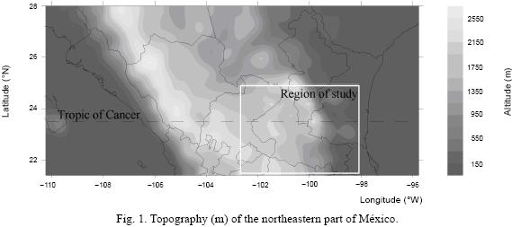
The northeastern part of México (Fig. 1) is a multifaceted region where local precipitation is governed by both topographic and atmospheric influences. Regionally, the physiography and the atmospheric circulation combine to create a spatially complex climatology, with strong seasonal contrasts (Comrie and Glenn, 1998). Thus, the big masses of humid air coming from the Gulf of México create an increase in the content of water vapor for the low altitude and coastal zones causing rainfalls and warm temperatures.

On the other hand, with the increase of altitude towards continental lands, these air masses lose humidity with a drop in temperature due to the orographic shade effect. This causes highlands of the Mexican Altiplano (Mesa del Centro) to experience few rainfalls with a mean annual precipitation of 300–500 mm (García, 1988). The Mexican Altiplano is characterized by warm dry to arid climates with typical semi–desert vegetation like grasslands and scrubland (Rzedowski, 1978).

Previous studies about climate regionalization in México have focused primarily on analysis of precipitation data in a coarse resolution (García, 1988; Comrie and Glenn, 1998; Giddings et al., 2005). For example, the standardized precipitation index (SPI) has been used to regionalize and classify precipitation zones based on quantity and seasonal variability of precipitation. SPI–zoning patterns can be useful in describing climatic phenomena such as ENSO (Giddings et al., 2005). However, there is a lack of studies in a finer–resolution scale for many regions of México despite the fact that they may offer more details about climate patterns associated with subtle topographic gradients. We use a combination of approximately 30 years of monthly mean temperature and precipitation data from 173 meteorological stations located in state of San Luis Potosí, México. These data were analyzed through PCA and geographical information systems (GIS) to distinguish among different climate and vegetation regions at this northeast zone of México.

In addition, we classified each of these climate regions based on the modifications introduced by Garcia (1988) to Koppen's classification system. Such amodification is important to obtain amore relevant description of climatic types taking into account many aspects on meteorological variability. The knowledge of a good regional climate classification finds several applications in fields such as agriculture, forestry, biodiversity, phenology, hydrology as well as environmental policies. Even though there exists a regional climate map for the Mexican territory in the Atlas Nacional de México (García, 1988), this is a coarse–resolution analysis based on dominant meteorological phenomena such as precipitation regimens and annual distribution of temperature (mentioned by Giddings et al., 2005). In contrast, we conducted PCA to describe the distribution of these patterns on a regional scale.

 

2. Methods

PCA is a multivariate statistical technique that involves linear transformations of a matrix of standardized observed variables, based on the eigenvalues and eigenvectors of either a correlation matrix or a covariance matrix (Ehrendorfer, 1987; Richman, 1981). The principal analytical purpose of PCA is to reduce the dimensions of the observed information, compiled in a data set, preserving the original data variability. Eigenvectors define a new coordinate system which is orientated in such a way that every new axis points to the maximum variability of the information (Wilks, 1995; Richman, 1981). It has been argued that the use ofthe correlation matrix, as opposed to covariance matrix, allows a direct comparison between dry and wet stations, but it is not useful to distinguish geographical effects (Comrie and Glenn, 1998). Therefore, we carried out PCA applying a covariance matrix. In this way, we obtained spatial patterns ofthe climatic variability.

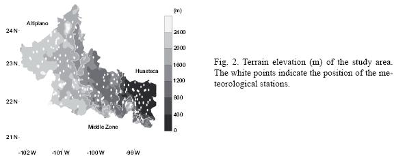
We used monthly means of precipitation and temperature from 1940 to 1997, obtained from México 's Comisión Nacional del Agua (CNA). A total of 173 stations were chosen throughout the study area, covering the region of San Luis Potosí, which is characterized by a strong topographic gradient (Fig. 2). According to the height above sea level, three principal geographical regions can be distinguished; the zone on the eastern side with altitudes below 500 m is called Huasteca. The Middle zone is located in altitudes varying between 500 m and 1,500 m, and finally the region on the western side, called Altiplano, with altitudes above 1,500 m.

The 173 stations included in the analysis had an average of 28 years of data. In order to carry out the PCA, the first step was to standardize the meteorological variables, forming a 24 x 24 covariance matrix (i.e., 24 monthly means: 12 for temperature and 12 for precipitation). For this, we applied the following formula:

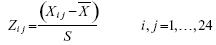
where each variable was standardized, so that each observation is expressed in terms of its difference from the mean, divided by the standard deviation.

The next step was to carry out a climate classification based on the Köppen criterion as modified by Garcia (1988). Köppen's system defines world climatic regions, based mainly on latitudinal effects. Consequently, the Köppen criterion may not correspond accurately to regional conditions, where changes in climate patterns are also due to altitudinal effects. This modified climatic classification was used subsequently to define bioclimatic zones based on vegetation data for two different temporal points. The vegetation data come from: 1) a land–use map developed by México' s Instituto Nacional de Estadística, Geografía e Informática (INEGI) obtained from aerial photographs at 1: 250,000 scale that represents vegetation cover in year 1976; and 2) an update of the previous dataset based on visual interpretation of space–maps derived from Landsat images, which represent vegetation cover in year 2000 (Palacio–Prieto et al., 2000). Each layer of vegetation was analyzed using GIS in order to find changes of regional vegetation patterns for every climate.

 

3. Results and discussion

 

3.1 Principal component analysis

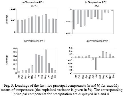
In Figure 3 we show the results for the covariance matrix of monthly means of the accumulated precipitation and temperature of 173 stations. We consider only the first two principal components because they explain 85 per cent of the variance. The analysis indicates an interesting distribution for the first principal component (PC1), showing an extraordinary precipitation period from June to September (Fig. 3c). Further, an inspection of the variability of the monthly accumulated precipitation, observed in PC1 axis, reveals that two principal seasons can be distinguished: a relatively dry period from October to May and a rainy season from June to September. The precipitation variability included in PC2 shows a dry period in early summer and a light to moderate rainfall in the rest of the year (Fig. 3d). This mid–year drought in early summer is associated with the known phenomenon called canícula/(dog days) (Magaña etal., 1999; Vázquez, 2000; Cavazos etal., 2002). In late fall and early winter, PC2 reflects the influence of hurricanes and events of El Niño Southern Oscillation (ENSO) (Cavazos and Hastenrath, 1990). The PC1 for temperature shows high variability from August to November with a maximum in September (Fig. 3a). It can also be concluded that, climatically, the most stable months are March and April. The variability observed in PC2 for temperature can be explained by cold fronts moving into the area between late summer and early winter (Fig. 3b).

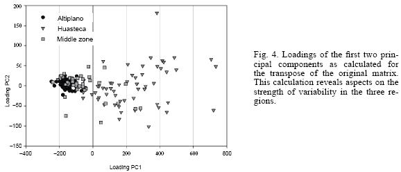
To obtain a geographical insight of the variability, we carried out PCA for the covariance matrix of the transpose of the original matrix. The monthly means of temperature and accumulated precipitation of 173 stations corresponds, in this calculation, to a 173 X 173 matrix. In Figure 4, we show the results for the transposed matrix. The variance explained by the first two components was 96.69 %. The stations were distributed principally along of the PC1 which was associated to precipitation variability. Noticeably, this variability coincided with the topographic gradient defined by the three main regional zones: Huasteca, Middle zone and Altiplano. In Figure 4, one can also see that the stations located in the Altiplano are closely grouped, i.e. the variability is relatively small. The maximum interannual precipitation variability is found in stations located in Huasteca. The seasonal variability of rain increases in the direction of Huasteca where the altitude is less than 500 m. Otherwise, in desert zones, large seasonal dry periods occur due to topographic effects and to the fact that the region is close to the Tropic of Cancer, i.e. a region where normally air descends. The PC2 was related to extraordinary events such as El Niño phenomenon, canícula periods and hurricanes. The stations with major variability are found in zones that can be affected by hurricanes.

 

3.2 Climate classification

The variety of climates inside a region is principally determined by geographical factors. Moreover, vegetation and land cover also play an important role in flows of energy and heat. The region studied in this research work exhibits large altitudinal contrasts. The Middle zone shows a gradient of altitude with an eastward transition from dry to humid climate. It creates environments that are characterized essentially by their geographical position, climate and typical vegetation (White and Hood, 2004). There is a clear spatial association between vegetation, climate and topography. For instance, arid climates are associated with highlands and desert vegetation. Low lands are related to humid temperate climates and tropical forest.

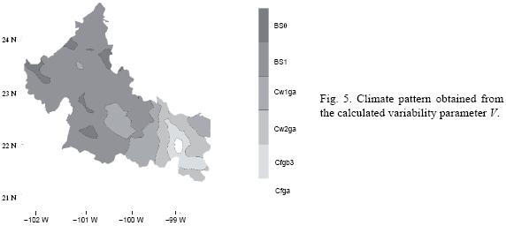
Since the region is characterized by a topographic and climatic complexity, it is difficult to find an appropriate regionalization method according to station distribution. We proceed as follows: once we have performed PCA of the transposed matrix of 173 x 173 elements, we calculated for each station the parameter V= (PC1) (Var1) + (PC2) (Var2), where PC1 and PC2 are the first two principal components, Var1 and Var2 are the corresponding explained variances and V is a measure of the variability. In this way, the stations are pondered according to the explained variance by the most important principal components. Stations located in a range of V will represent a range of climatic variability. Once we have the spatial distribution of V, we carried out an interpolation over the whole region applying a kriging method. Based on climate classification, six different regions were determined (Fig. 5).

Once we have obtained the climate regionalization, the following step was to carry out a climate classification. We applied Garcia's (1988) modified version of the climate classification system of Köppen. In Köppen's system, the regional level of temperature anomalies is smaller than that considered by García for the central–northern part of México. García found an acceptable empirical relationship between sub–type of climates and a climate distribution, based on meteorological data. Therefore, we considered the same classification criteria for our statistic results of the region of San Luis Potosí, as shown in Figure 5.

Humid stations present a climate classified as humid temperate with rains the whole year (Cfga). The precipitation in the humid season should not be larger than ten times the highest monthly precipitation and less than three times the driest monthly precipitation. Regions satisfying these conditions are located in Huasteca, where the warmest monthly mean of temperature reach values larger than 22 °C (Fig. 6a).

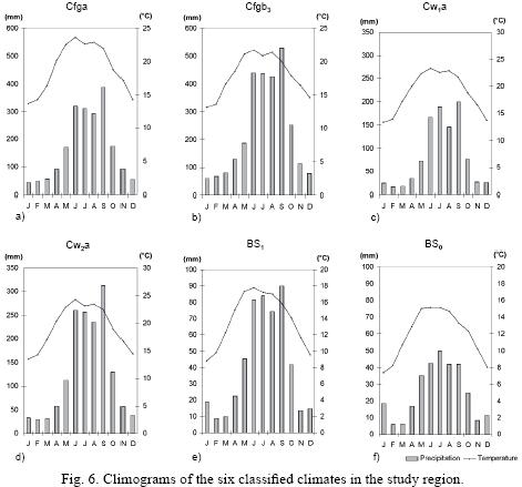
A further refinement of the climate humid temperate with rains the whole year is represented by (Cfgb₃). It has the same rainfall classification as the previous one, but with at least four monthly mean temperatures larger than 10 °C. This kind of climate is also found in the Huasteca region (Fig. 6b).

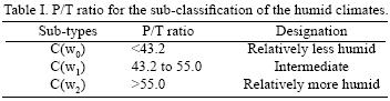
Two types of climates can be distinguished in the Middle zone. sub–humid temperate with rains in summer season. For the sub–classifications w₁ and w₂ we applied García's criterion of the ratio (P/T) of the total rainfall and the average temperature (Table I). In Cw1ga climate, the rainfall for the most humid month in summer should be larger than ten times that of the driest month and it must be larger than 40 mm. The coldest monthly mean temperature should be between –3 and 18 °C. In addition, the annual average temperature should be larger than 10 °C and the maximum temperature for the hottest month should be larger than 22 °C (Fig. 6c). The Cw₂ga climate belongs to the same classification, but it is typified by more humidity (Table I and Fig. 6d).

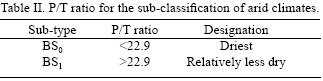
Two sub–types of dry or arid climates (BS₀, BS₁) are found in the zone of Altiplano. They are characterized by low rainfall, less than 500 mm, in the summer season. According to García's criterion, the subdivision is done using the relation P/T as an indicator of the degree of dryness (Table II and Figs. 6e, 6f).

 

3.3 Bioclimatic regions

The term bioclimatic region has been adopted in this study to include the elements of both vegetation and climate. Vegetation zones have been defined by several criteria such as physiognomy and floristic composition. They show a strong relationship with climate (Karlsen and Elvebakk, 2003; Hessburg etal., 2005; Piovesan etal, 2005). Defining such bioclimatic zones is important because the modification of land use and cover may produce a direct effect on regional climate change by altering the physical parameters that determine the absorption and disposition of energy at the Earth's surface (Feddema etal., 2005).

Dry climates (BS) represent 66 % of the whole surface of the study area and are localized principally in the Altiplano region where topographic and altitude effects play an important role. This dry climate is associated with desert vegetation such as desert shrublands, arid grasslands and dry woodlands (chaparral after Rzedowski, 1978) to a less extent. Temperate climates represent 26 % of the whole State surface and are localized in the Middle zone. Characteristic vegetations of this kind of climate are perennial forest (mainly pine–oak forests) and some patches of deciduous tropical forest. There are some regions with semi desert shrublands but these represent only 3 % of the whole area of Cw climates. Finally, humid temperate climates (Cf) correspond to only 8 % of the whole study area and are localized in the low lands close to the Gulf of México, in the Huasteca region. Humid vegetation types are dominant in this zone.

We now discuss these concepts for the region of the state of San Luis Potosí, as shown in Figure 7. It reveals rather coarse–resolution vegetation types because we had to merge similar plant community classes (all shrublands, for instance) in order to reduce our original matrix (climate vegetation). A detailed and rigorous land use and cover change study is beyond the objectives of this study. Instead, we highlight pervasive and important trends in unsustainable land use change practices (exemplified by conversion of desert vegetation into croplands) and changes in vegetation which could point to effects of climate change. We proceeded as follows: applying the classification of the six climates BS₀, BS₁, Cfga, Cfgb₃, Cw₁ga and Cw₂ga in combination with information on types of vegetation, we defined 85 bioclimates in the study region. It is worth mentioning that the vegetation types varied from climate to climate, with Cw₁ga having the largest number of bioclimates. By comparing 1976 and 2000 images, we were able to assess the relative change in each bioclimate with respect to its original extension as well as to look for spreading of vegetation from one climatic zone into another. The results of this analysis are given in Figure 8, where the vertical axis represents the order of magnitude (in %) in which the bioclimates varied. A positive (negative) % means an increase (decrease) in area of the corresponding bioclimate, represented in the horizontal axis. Whereas most of the bioclimates showed little change between the two considered years, we find an increase of human induced vegetation such as croplands and secondary grasslands associated with a decrease of woody cover in most of the climatic regions of San Luis Potosí (Fig. 8). For instance, in the humid zone, rainfed agriculture in the Cfga climate (Huasteca region) increased 470 % and induced grasslands increased more than 3000 % in the driest region (BS₀) during the 24 –year period. These two examples of extreme bioclimatic changes are not depicted in Figure 8 because the scale of the vertical axis would be too large. Rainfed agriculture also increased 190 % in Cw₂ga and 107 % in Cw₁ga climates (Fig. 8). While humid temperate climates (Cf) represent only 8 % of the whole study area, vegetation associated with these climates has changed dramatically as shown for zones 1, 3 and 6 (Fig. 7a and 7b, and Fig. 8).

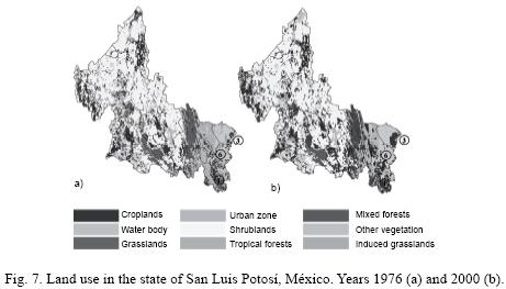
Decline is also outstanding in tropical seasonal evergreen forest in Cw₂ga climate (–70 %) and tropical deciduous forest in Cw₁ga (–78 %). These land cover changes are likely to modify the long–term climate by altering the solar energy balance and to have effects on other regional climatic variables such as precipitation (Lean and Warrillow, 1989; Shukla et al., 1990). However, we are aware that the effects of land–cover change on climate are not well understood because regional impacts are not correctly represented in annual global statistics (Feddema et al., 2005). Increases in natural vegetation were also noted mainly in the arid regions, where shrublands are occupying areas previously devoted to croplands. For instance, in BS₀ climate mesquite shrublands increased by 130 % and creosote bush shrublands by 39%.

 

4. Conclusions

We use a combination of nearly 30 years of monthly means of temperature and precipitation data from 173 meteorological stations to carry out a climate classification of the state of San Luis Potosí, México. PCA statistical technique has been widely used for climatic regionalization although it has seldom been applied to more than a single variable. We applied PCA to a covariance matrix formed by two meteorological variables, precipitation and temperature. We obtained information on the annual variability of climate in the region. In contrast, the PCA for the covariance matrix of the transpose of the original array revealed a spatial distribution of the variability. These two PCA were useful for regionalizing complex topographic zones with a large rainfall variation and permitted the classification of climate in the study area. The results of our analysis revealed that spatial patterns of climate variability, vegetation and topography are fairly similar. This is a good indication that climate and vegetation in this strong topographic gradient is determined by the altitude. The calculation of PC1 and PC2 indicates that climate variability is closely related to mean annual precipitation and extraordinary climate events. These atmospheric phenomena influence regional climate patterns due to their seasonal frequency. By applying the classified climates and types of vegetation, 85 bioclimatic zones were defined. The comparison of satellite images from the years 1976 and 2000 allowed estimating how these bioclimates have evolved in this period. Finally, the next step in our investigation is to extend this study to the whole area of México.

 

Acknowledgements

The authors want to thank CONACYT, IPICYT and Fondos Mixtos CONACYT–SLP (FMSLP–02–5627) for the financial support of this research work. We are also grateful to Servicio Meteorológico Nacional and Comisión Nacional del Agua of México for providing the meteorological data. We also appreciate the comments of two anonymous reviewers.

 

References

Cavazos T. and S. Hastenrath, 1990. Convection and rainfall over México and their modulation by the Southern Oscillation. Int. J. Climatol. 10, 377–386.        [ Links ]

Cavazos T., A. C. Comrie and D. M. Liverman, 2002. Intraseasonal variability associated with wet monsoons in southeast Arizona. J. Climate 15, 2477–2490.        [ Links ]

Comrie A. C. and E. C. Glenn, 1998. Principal components–based regionalization of precipitation regimes across the Southwest United States and Northern México, with an application to monsoon precipitation variability. Clim. Res. 10, 201–215.        [ Links ]

Ehrendorfer M., 1987. A regionalization of Austria's precipitation climate using principal component analysis. J. Climatol. 7, 71–89.        [ Links ]

Feddema J. J., K. W. Oleson, G. B. Bonan, L. O. Mearns, L. E. Buja, G. A. Meehl and W. M. Washington, 2005. The importance of land–cover change in simulating future climates. Science 310, 1674–1678.        [ Links ]

García E., 1988. Modificaciones al sistema de clasificación climática de Kóppen. Offset Larios, México, D. F.        [ Links ]

Giddings L., M. Soto, B. M. Rutherford and A. Maarouf, 2005. Standardized precipitation index zones for México. Atmósfera 18, 33–56.        [ Links ]

Hessburg P. F., E. E. Kuhlman and T. W. Swetnam, 2005. Examining the recent climate through the lens of ecology: Inferences from temporal pattern analysis. Eco. Appl. 15, 440–457.        [ Links ]

Karlsen S. R. and A. Elvebakk, 2003. A method using indicator plants to map locale climatic variation in the Kangerlussuaq/Scoresby Sund area, East Greenland. J. Biogeography 30, 1469–1491.        [ Links ]

Lean J. and D. A. Warrillow. 1989. Simulation of the regional climatic impact of Amazon deforestation. Nature 342, 411–413.        [ Links ]

Magaña V., J. A. Amador, and S. Medina, 1999. The midsummer drought over México and Central America. J. Climate 12, 1577–1588.        [ Links ]

Malmgren B. A. and A. Winter, 1999. Climate zonation in Puerto Rico based on principal components analysis and an artificial neural network. J. Climate 12, 977–985.        [ Links ]

Mestas–Núñez A. M., 2000. Orthogonality properties of rotated empirical modes. Int. J. Climatol. 20, 1509–1516.        [ Links ]

Nieto S., M. D. Frías and C. Rodríguez–Puebla, 2004. Assessing two different climatic models and the NCEP–NCAR reanalysis data for the description of winter precipitation in the Iberian peninsula. Int. J. Climatol. 24, 361–376.        [ Links ]

Palacio–Prieto J. L., J. López–García, G. Bocco, M. Palma, A. Velázquez, I. Trejo–Vázquez, J–F. Mas, A. Peralta, F. Takaki–Takaki, J. Prado–Molina, A. Victoria, A. Rodríguez–Aguilar, L. Luna–González, R. Mayorga–Saucedo, G. Gómez–Rodríguez and F. González, 2000. La condición actual de los recursos forestales en México: resultados del Inventario Forestal Nacional 2000. Boletín del Instituto de Geografía de la UNAM, Investigaciones Geográficas 43, 183–202.        [ Links ]

Piovesan G., F. Biondi, M. Bernabei, A. Di Filippo and B. Schirone, 2005. Spatial and altitudinal vegetation zones of the Italian peninsula identified from a beech (Fagus sylvatica L.) tree–ring network. Acta Oecol. 27, 197–210.        [ Links ]

Rzedowski J., 1978. La vegetación de México. Limusa, México, 432 pp.        [ Links ]

Richman M. and P. J. Lamb, 1985. Climatic pattern analysis of 3 and 7 day summer rainfall in the central United States: some methodological considerations and a regionalization. J. Clim. Appl. Meteorol. 24, 1325–1343.        [ Links ]

Richman M., 1981. Obliquely rotated principal components: an improved meteorological map typing technique. J. Appl. Meteorol. 29, 1145–1149.        [ Links ]

Shukla J., C. Nobre and P. Sellers, 1990. Amazon deforestation and climate change. Science 247, 1322–1325.        [ Links ]

Vázquez M. C., 2000. Intraseasonal variation of convective activity in México and Central America. Atmósfera 13, 95–108.        [ Links ]

White D. and C. Hood, 2004. Vegetation patterns and environmental gradients in tropical dry forests of the northern Yucatán peninsula. J.Veg. Sci. 15, 151–160.        [ Links ]

Wilks, D. S., 1995. Statistical methods in the atmospheric sciences. Academic Press, San Diego, CA, 464 pp.        [ Links ]