Convective rainfall rate multi–channel algorithm for Meteosat–7
and radar derived calibration matrices

 

A. LUQUE
Grupo de Meteorología, Departamento de Física, Universitad de les Illes Balears (UIB),
Palma de Mallorca, España
Corresponding author e–mail: angel.luque@uib.es

I. GÓMEZ
Departamento de Proyectos, Instituto Nacional de Meteorología (INM), Madrid, España

M. MANSO
Departamento de Teledetección, Instituto Nacional de Meteorología (INM), Madrid, España

 

Received November 5, 2005; accepted January 12, 2006

 

RESUMEN

El algoritmo llamado CRR (Convective Rainfall Rate) ha sido desarrollado para detectar células convectivas mesoescalares y para monitorizar la precipitación asociada más probable. Es capaz de estimar intensidad de precipitación utilizando los tres canales del Meteosat–7 y matrices calibradas con datos de radares terrestres de precipitación. Estas matrices de precipitación han sido construidas a partir de las técnicas Rainsat pero combinando las dos bandas infrarrojas para favorecer la detección de nubosidad convectiva. Además, éstas han sido desarrolladas al norte del continente europeo sobre los países bálticos con datos de radar del proyecto Baltex proporcionados por el SMHI (Swedish Meteorological and Hydrological Institute) y al sur de Europa, sobre la Península Ibérica con datos de radar proporcionados por el INM (Instituto Nacional de Meteorología). En este trabajo se valida el método empleado de calibración de las matrices del CRR, se realiza un análisis de las matrices obtenidas al norte y sur de Europa, y finalmente una serie de imágenes CRR se verifican de forma cualitativa con respecto a las imágenes de radar.

 

ABSTRACT

The CRR (Convective Rainfall Rate) algorithm was developed to detect intense mesoscale convective cells and to screen the most probable precipitation associated. It estimates rainfall intensity using the three bands of the Meteosat–7 and matrices calibrated with earth–based radars. Calibration matrices were performed following an accurate version of the Rainsat techniques but combining the infrared bands to detect convective clouds. Matrices were developed, up for the North of Europe, over the Baltic countries, with data from the radar of the Baltex Project provided by the SMHI (Swedish Meteorological and Hydrological Institute) and for the South of Europe, over the Iberian Peninsula, with radar data as provided by the INM (Spanish Meteorological Institute). In the present research, the CRR calibration methodology is validated, an analysis of calibration matrices differences in both areas over Europe is detailed and CRR resulting images are verified in a qualitative manner using rainfall radar images as ground true.

Keywords: CRR, rainsat, meteosat, convective rainfall rate, satellite estimated rainfall, radar, calibration matrices, satellite rainfall algorithm.

 

1. Introduction

Real time rainfall estimation using geosynchronous satellite data has several applications in meteorology and hydrology. Although the estimates are indirect, the high frequency and high spatial resolution of the measurements, as well as the broad area that they cover, make them uniquely complementary to rain gauge and radar measurements (Vicente et al., 1998). Conventional rain gauges, when they exist, have mostly a sparse distribution and data are not usually available in real time. On the other hand, meteorological radars have a limited spatial coverage and are usually affected by attenuation problems, beam overshoot or ground and mountain echoes. However satellite derived rainfall rate estimates are available every 30 minutes (10 minutes for Meteosat rapid scan) at a 7–km spatial resolution over Europe and thus can assist in the detection of flash flood and heavy precipitation areas in real time.

The development of visible and infrared techniques has a long history and relies upon the relationship between cloud–top characteristics and the rainfall falling from their bases. Under this focus, many algorithms have been developed. One of the most simple mono–spectral method and widely used is the GOES (Geoestationary Operational Environmental Satellite), precipitation index (GPI; Arkin and Meisner, 1987). The technique screens the fraction of cloud colder than 235 °K in the infrared with a fixed rain rate. More complex algorithms such as the Auto–Estimator (Vicente et al., 1998), uses the GOES–8 and –9 in the infrared 10.7 µm band to compute real–time precipitation amounts based on a power–law regression algorithm. This regression was derived from a statistical analysis between surface radar rain rate estimates and satellite infrared cloud top temperatures collocated in time and space.

Bi–spectral methods as suggested by the Rainsat techniques are supported on IR/VIS (Infrared/ visible) matrices (Lovejoy and Austin, 1979; Bellon et al., 1980). These methods screen out cold but not highly reflective clouds or those that are highly reflective but have a relatively warm top. The algorithm is based on a supervised classification trained by radar to recognize precipitation from visible brightness and infrared cloud top temperature. Results of an optimization of Rainsat using Meteosat over the United Kingdom were published (Cheng et al., 1993; Cheng and Brown 1995). In this work some correlation methods between radar and satellite data were designed based on a statistical spatial optimization of the estimated rainfall area with the radar rainfall area. The role of visible data in improving the rainfall estimates was also examined by King et al. (1995) their results showing a higher correlation with validation data using VIS/IR over the IR alone for the case of warm orographically induced rainfall. For cold, bright clouds the correlations are similar.

The CRR technique uses the three Meteosat–7 bands, and earth radar derived calibration matrices to detect and estimate convective rainfall precipitation from mesoscale convective systems over Europe. Calibration tables were generated based on the empirical relationship than the higher and thicker are the observed clouds, the higher is the probability of occurrence and the intensity of precipitation. Information about cloud top height and about cloud thickness can be obtained, respectively, from the infrared brightness temperature and from the visible counts (Scofield, 1987; Vicente and Scofield, 1996). Additionally, the brightness temperature difference between the 11 µm and 6.7 µm channels was used in the calibration process because it is an useful parameter to detect highly developed convective cloudy cells (Kurino, 1997). Infrared water vapour band was found to be important in convective processes since stratospheric water above deep convective clouds has been identified from Meteosat observations in the infrared window and water vapour bands (Schmetz et al., 1997). It was demonstrated that the equivalent brightness temperature in the water vapour can exceed that in infrared window by several degrees because of stratospheric water vapour above clouds top.

The spatial correlation between radar and satellite has a capital importance in the present research and two processes were applied. In first place, as the European continent is distributed over mid and high latitudes, the correction of the parallax effect (Vicente et al., 2002) is essential. Secondly, a spatial fit in 15 x 15 pixel zones of the satellite image around the significant radar pixels attempting to find the maximum spatial correlation between areas of maximum radar reflectivity and minimum brightness temperature.

Long–term convective calibration matrices of two and three dimensions are performed in both ends of Europe using a technique in which a validation method is also designed. CRR output images are evaluated in a qualitative manner comparing with radar images over Spain in September and October of 2002, and over the Baltic Sea in June and July of 2000. At the end of the work, the most outstanding differences between calibration matrices are detailed and discussed.

 

2. Data used

The matrices for the Iberian Peninsula were calibrated using earth based radars in mmh^–1 and echo–top radar of cloudy tops height in km. Both datasets come from the Spanish radar network belonging to the INM. They are focused on 40° N and 3° W, with 512 by 512 pixels size and 4 km spatial resolution. Radar images are generated operationally every 10 minutes and were selected for the present research corresponding with convective rainfall episodes between 1999 and 2001, preferably during spring, summer and part of autumn.

Matrices of the Baltic area were calibrated using rainfall earth radar in mmh^–1 from the Baltic radar network, every 15 minutes, provided by the SMHI (Swedish Meteorological and Hydrological Institute). The radar images are focused on 57.3° N and 18.4° E, 550 by 900 pixels size and 2 km spatial resolution. They were selected during rainy days in June and July 2000 as shown in Table I.

The lower radar CAPPI (Constant Altitude Plan Position Indicator) at 2.5 km altitude, registered in reflectivity (Dbz) units was transformed into rainfall intensity in mmh^–1 using the Marshall–Palmer Z–R relation, which recommended coefficients for general rain type over mid–latitudes are: a=200, b=1.6 (Marshall and Palmer, 1948).

The Meteosat–7 data used in this work are: infrared band brightness temperature in degrees Kelvin T_IR(°K) (λ_IR=10.5–12.5 µm, 5 by 5 km resolution), infrared water vapour band in degrees Kelvin T_WV (°K) (λ_WV=5.7–7.1 µm, 5 by 5 km resolution) and the visible channel in brightness counts (λ_VIS= 0.4–1.1 µm, 2.5 by 2.5 km resolution). Normalized visible counts are obtained for all day pixels dividing by the cosine of solar zenith angle (Binder, 1988).

The Meteosat data are contained in images from EUMETSAT which cover Europe, every 30 minutes. Note that resolution is referred to satellite nadir, this magnitude change with latitude and longitude for geostationary satellite image original projection.

 

3. Methodology

3.1 Rainfall matrices calibration

The fundamental algorithm consists basically of obtaining two frequency distributions by correlating spatially simultaneous radar data with the satellite data in order to discriminate between raining and non–raining clouds (Bellon et al., 1980).

As shown in Figure 1, for the general case of diurnal 3–D matrix generation (using the three Meteosat bands), the first step involves a spatial and temporal correlation of radar and satellite data. When this problem is solved (see the next subsection), every radar pixel of convective rainfall intensity (R_CINT) is corresponded with every value of the three bands of the satellite in physical units such as: T_IR, T_WV and normalized count of the visible band (Vc). The echo–top image was used in the Spanish array calibration process to locate pixels with and without rainfall linked to high clouds tops and, therefore, potentially convective points. A rain radar point (R_INT) associated to a echo–top value greater than six kilometres above sea level (H_E–T > 6 km) is considered a convective rain radar point (R_CINT). This simple criteria have been used successfully by the INM for many years with unstable weather over the Iberian Peninsula. Qualitative observations not shown in this paper demonstrated the efficiency of the method comparing ground–based lightning images and satellite infrared images with active clouds cold tops. Over the Baltic area this correlation between convection and high altitude radar echoes has not been clearly found and no convective threshold has been applied for radar images. For this first research, authors believe in the benefits of the dynamical radar–satellite spatial correlation and in the statistics of CRR calibration method with the resulting probability matrix and the EQ_PC parameter to separate rain from no rain areas in the rainfall matrices.

The next step was the development of three arrays: two for frequencies (rain and no rain) and one for accumulation (accumulated rain). In Figure 1 it can be seen how each array has three orthogonal axes which represent the satellite data: Vc, T_IR – T_WV and T_IR. The horizontal axis (T_IR – T_WV) is the remainder between T_IR and T_WV, it is represented by ΔT_IR in equations. The rain matrix is a frequency array of rainfall cases, which represents a total number of radar–satellite points with rainfall rate greater than 0 mmh^–1 (R_CINT > 0). The no rain matrix represent a frequency of radar points with no rainfall (R_CINT = 0). The accumulated rain matrix is a radar rainfall accumulation array, in which, every value of radar rainfall intensity is added. In short, radar data is classified by the satellite magnitudes in matrices. In such a way, elements of rain and no rain frequency arrays are represented, respectively, by F_R(Vc, ΔT_IR, T_IR) and F_NR(Vc, ΔT_IR, T_IR). Every element of the accumulated rain matrix is also represented by SR_CINT(Vc, ΔT_IR, T_IR).

The rainfall probability matrix (P_R) is calculated by rain and no rain arrays elements expressed by the relation:

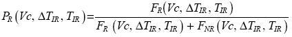.......................(1)

where F_R(Vc, DT_IR, T_IR) + F_NR(Vc, DT_IR, T_IR) is the total number of rainfall and no–rainfall cases associated to the satellite data.

The mean rainfall array is made using the following criteria: array elements with rainfall probability lower than a defined probability variable called as EQ_PC and explained in section 3.3, are put to zero (R_CINT=0). If they have a rainfall probability greater than the EQ_PC, the mean rainfall intensity for each element is computed as shown in the next expression.

.....................(2)

For the nocturnal array or 2–D matrix, the process is similar but, without using the visible counts. The result is an array made only with the two Meteosat infrared bands, in which the vertical axis is T_IR and the horizontal ΔT_IR (or T_IR – T_WV) as can be seen in Tables II and III.

 

3.2 Temporal and spatial correlation

Every radar and satellite images (inside the dotted box in Fig. 1) were correlated for a time lapse no greater than 5 minutes. Collocated radar–satellite datasets were distributed every 30 minutes in the calibration process (t – t₁ = 30 min in Fig. 1), corresponding with heavy convective rainfall days.

The spatial correlation was thought to keep the quality and resolution of radar data through the process; it was decided to remap satellite images to radar projection, resolution, size and image centre. Satellite remapped points are corrected spatially (lat*, lon*) with respect to radar pixels (lat, lon) after two steps: The first one is the parallax correction (Vicente et al., 2002) and the second one, displacements of 15 x 15 pixel areas in search of maximum correlation around radar pixels. To complete the second process radar reflectivity is transformed to rainfall rate by the Marshall–Palmer relation, and satellite T_IR are transformed using a satellite algorithm. Over the Iberian Peninsula a satellite rainfall image was estimated using a bi–spectral IR/VIS matrix. Over the Baltic area an IR/VIS array is not known, so the preceding rainfall image was computed via Auto–Estimator technique (Vicente et al., 1998), adapted to the European region (Vicente, 2001). The maximum spatial correlation is obtained by carrying out slight spatial displacements of the satellite rainfall 15 x 15 pixels clusters around the significant radar pixels. Translations that provide greatest correlations coefficients are selected and applied then to modify each satellite pixel position (INM, 2000).

 

3.3 Validation of the method

The matrices calibration technique described in this work can be evaluated using statistics indexes, such as: EQ_PC (Probability of equal satellite–radar rain area), POD (Probability of Detection), FAR (False Alarm Ratio) and CSI (Critical Success Index). They are calculated using data stored in matrices as follows:

The EQ_PC is the probability level that matches the total number of radar rain points with satellite rain points. To compute this factor has been selected as radar rain points, those points stored in the rain matrix. In addition, the total number of radar rain points is the total number of points in the rain matrix and it is called N° R (Eq. 3 and the 2–D rain matrix in Table II–A). On the other hand, there has been selected, as satellite rain points, those stored in the rain and no rain matrices. Radar and satellite rain points in matrices are linked to a rain probability value performed in the probability array (Eq. 1). For every probability value (P) the total number of satellite points (TSAT) is accumulated from higher to lower probability as shown in the expression (4).

...............................................(3)

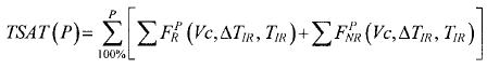..................(4)

where

represent the sum of all the matrices elements.

TSAT(P) is compared with N° R from highest probability (P = 100%), where N° R is bigger than TSAT(P), to lowest (P = 0 %), where N° R is smaller than TSAT(P). The probability value in which TSAT(P) is closer to N° R then EQ_PC = P. The probability level has been reached and the total number of satellite rain points in matrices is the same than the total number of radar rain points.

To calculate POD, FAR and CSI a contingency table (Marzban, 1998) have been performed for each matrix, as follows:

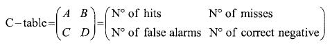
A, is the number of hits or number of radar rain points correctly detected by CRR. Using the matrices, A is the number of rain points from the rain matrix with probability greater than the EQ_PC. B, is the number of misses or number of radar rain points not detected by CRR. It is the number of rain points from the rain array with probability smaller than the EQ_PC. C, is the number of false alarms or number of radar no rain points estimated as rainy by CRR. Using the matrices, it is the number of no rain points from the no rain array with probability greater than the EQ_PC variable. D, is the number of correct negative or total number of radar no rain points correctly estimated by the CRR. POD, FAR and CSI are easily calculated as:

.............................................(5)

........................................(6)

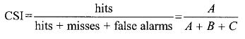...................(7)

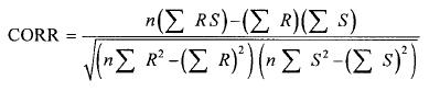
On other hand correlation coefficients were performed for every set of radar (R) and pre–estimated Rainsat image (S) in mmh^–1 following the equation (8) where 'n' is the total number of R and S pair of points:

..........(8)

 

4. Results

4.1 Rainfall matrices

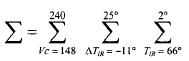
The calibration matrices developed for the Iberian Peninsula and for the Baltic Sea can be both, 2–D useful during night time and 3–D to be applied in daytime. It has been considered daytime for points where sun zenith angles are smaller than 80°. The 2–D arrays have two axes corresponding respectively to: T_IR as a vertical axis, from –66 to 2 °C each 2 degrees and T_IR – T_WV as horizontal axis, from –11 to 25 °C each 2 degrees (tables II–D and III). The 3–D arrays include, besides, a third axis, composed by Vc from 148 to 240, each 4 counts as shown in tables IV and V. In those tables the 3–D matrices are partially represented and for every T_IR valcue, the V whole range is viewed along the vertical axis.

The matrices elements are rainfall classes derived from rainfall intensities in mmh^–1 as shown in Table VI. Multiplying every rainfall class by 24, they are scaled to 8–bit count range (0–255) used in the final CRR output images as shown in figures 3 and 5. The CRR images were generated from a simple classes association extracted from matrices and satellite parameters.

In Table II the resulting 2D rain (A), no rain (B), probability (C) and mean rainfall (D) arrays performed over the Iberia Peninsula are shown. The rain and no rain tables with the number of rain N° R and no rain N° NR points reveal the size of the samples used to develop the algorithm. The probability table shows in grey colour cells with probability higher than the EQ_PC parameter and therefore, CRR rain points.

 

4.2 CRR images, qualitative observations

Figures 3 and 5 are the CRR graphic output derived from satellite and matrices calibrated over the Iberian Peninsula and the Baltic Sea, respectively, shown by way of example. CRR has been conceived principally to aid short–term weather prediction and timely production is of major importance. It was therefore decided to process all different data on a common spatial resolution and compare the different dataseis in a qualitative way. Some convective cases in September and October of 2002 over the Iberian Peninsula and in June and July of 2000 over the Baltic Sea were checked with radar data. It has been observed that CRR images give a suitably clear idea of the position and intensity of cloudy convective cell with heavy rainfall and cold tops. Nevertheless, using only 2–D or night matrices, rainfall areas located via CRR are spatially overestimated in most of cases and maximum rainfall areas are slightly displaced with respect to radar maximum rainfall zones. In addition, 2–D CRR has a general tendency to undervalue rainfall intensity with respect to radar precipitation. Checking 3–D matrices CRR images, the spatial correlation between radar and CRR rain areas are better than using 2–D matrices, although close to midday hours 3–D CRR tends to underestimate precipitation.

A negative effect observed in 3–D CRR images during daytime with high solar zenith angles is noisy rainy spots with considerable rain intensity. Nevertheless, a significant spatial correspondence between the rainfall measured by radar (Figs. 2 and 4) with the corresponding approximated by the CRR algorithm (Figs. 3 and 5) has been observed in most of the cases. These figures are examples of heavy mesoscale convective events which common characteristic is the difficult to forecast with same precision by weather services. Figure 2 is a radar image of rainfall intensity for the Iberian Peninsula on October 9, 2002, at 6:50. At that time, there were storms of varying intensity over Catalonia and the maritime area north of the Balearic Islands, with maximum rainfall intensity around 13 mmh^–1. At 8 in the morning, news was given with respect to flooding in places on the metropolitan area of Barcelona city. Figure 3 is a CRR image with the same geographical characteristics as the radar image although ten minutes later (Fig. 2). The estimated rainfall intensity is shown as calculated from Meteosat–7 data and the 2–D matrix performed for the Iberian Peninsula (Table IV). Maximum values of 13 mmh^–1 are also observed, although CRR rain areas are over estimated. Figure 4 is a radar image of the Baltex Radars Network over the zone of the Baltic Sea to the south of the Scandinavian Peninsula and Denmark on the 21st June at 14:00. In this image, clear signs of moderate rainfall over Sweden are shown. Figure 5 is the CRR image generated over the same geographic area and same UTM time as the radar image (Fig. 4) using Meteosat–7 data and the 3–D array for the Baltic Sea (Table V). In spite of geostationary satellite pixel deformation due the high latitude (60° N) after been remapped to radar projection, a big spatial correlation with radar rainfall can be observed.

 

4.3 Two dimensional matrices differences

Clear differences between rainfall classes and their distribution were found after been analysed the Baltic and Spanish 2–D arrays together. Main classes were located in the Spanish matrix (Table II–D) between values of T_IR from –66 to –58 °C and between T_IR– T_WV from –11 to –3 °C. This result suggests that among these cold infrared brightness temperatures clouds tops are the highest, convection is very developed and meteosat pixel mean rainfall may be around 10 mmh^–1 (transforming classes in Table II–D to rainfall rate according to Table VI). Whereas the 2–D rainfall array performed over the Baltic Sea (Table III) does not show a clear convective cluster, since, the maximum rainfall intensity is not above 5 mmh^–1 in any point.

With regard to the rain elements distribution, these are found mostly on the diagonal of matrices. Table VII was made to visualize differences in the distribution of classes between the Baltic and Spanish arrays. In this table, cells in light grey with 'Bt' letters correspond to classes of the Baltic matrix, cells in black are classes of the two matrices and cells in dark grey with 'Sp' letters are classes from the Spanish array. It can be seen that there are no 'Sp' cells, which implies that Spanish classes are all covered by the Baltic ones. Furthermore, since some 'Bt' cells are observed along the distribution diagonal edge, the Baltic matrix has a distribution of classes broader than the Spanish one.

 

4.4 Three dimensional matrices differences

To study the effect of the visible band on the matrices, a change was done in the structure with respect to the make–up shown in tables IV and V. In the new vertical axis configuration, for each visible normalized count (Vc), the complete T_IR range is shown every 4 degrees. Hereby, changes on rain elements distribution in a matrix structure similar to the 2–D array can be observed by increasing Vc. Tables VIII and IX show partially the new scheme and significant rain classes are shaded using two grey colours. Classes between 4 and 5 in light grey symbolize moderate rainfall from 3 to 7 mmh^–1 according to Table VI. Classes between 6 and 8 in dark grey indicate heavier rainfall from 7 to 20 mmh^–1 as shown in Table VI. Comparing the 3–D Spanish and Baltic matrices significant differences in class values and in the distribution have also found.

In the Spanish 3–D matrix it is observed a remarkable convective array area with class values above 4 which evolves along the visible range. This area grows slowly in number and intensity from Vc = 188, reaching a maximum for Vc = 224 with rain classes around 8 (17 mmh^–1, according to Table VI). Then this cluster decreases quickly in size and intensity until it disappear for Vc = 240. Table VIII shows part of the Spanish 3–D matrix where the highest rainfall clusters are located.

In the Baltic 3–D matrix, it can be observed a much less intense cluster of classes where, in no case, class values are above 4. This group grows slowly in size from Vc = 168 reaching a maximum for Vc = 188 and then it decreases gradually to Vc = 204. Table IX shows the place in the Baltic 3–D matrix where maximum rainfall clusters are located.

With respect to the distribution of classes, grey shaded tables analogous to Table VII, showing the overlap of 3–D matrices classes were made (tables X and XI). As Vc increases from 164 to 188, the diagonal distribution of classes in the Spanish 3–D matrix begins to broaden vertically on the left and to narrow on the right (Table X, shape of the group of 'Sp' cells plus black cells). This trend continues through to the end of the visible range although with a slight displacement of the distribution downwards and to the right. When Vc = 232 is reached, the Spanish distribution of classes is found to be very compact (Table XI, 'Sp' plus black cells).

The distribution of classes in the 3–D matrix over the Baltic Sea preserve a diagonal shape along the whole range of the visible band from 148 to 208 (Table X, 'Bt' plus black cells). Then it begins to narrow and taper out from left to right until the distribution disappears completely for Vc = 232 (Table XI, 'Bt' plus black cells).

 

5. Discussion

A spatial adjustment have been done between radar and satellite rainfall looking for the maximum correlation coefficient in pixel zones, the resulting matrices can be analyzed by spatial statistics as POD, FAR and CSI magnitudes. The best spatial correspondence has been obtained for the Spanish 3–D array (Table IV) according to the highest POD and CSI and the lowest FAR. Then comes the Baltic 3–D matrix (TableV) with the second better result and, finally, the two 2–D arrays (tables II–D and III). Mean correlation coefficients are around 0.4 for both 3–D matrices and around 0.3 for the 2–D arrays. These results suggest that it is positive to use visible band information in the calibration process for the daytime matrices.

One key question raised in this work was the selection of the calibration period to perform a long term calibration matrix. Selecting the greatest possible amount of radar and satellite data to develop the matrices over the Iberian Peninsula, statistics changed into satisfactory margins and classes have a tendency to converge to specific values and specific array positions. However, Baltic arrays classes have a tendency to drop to zero and to disperse to a broader distribution. That can be caused by one hand, the geostationary satellite pixel degradation due to remapping requirements on high latitudes and by the other hand, the scarce of convective rainfall in contrast to stratiform rain type over the Baltic area, even during the summer period. A shorter calibration period seems to be necessary to develop the best Baltic arrays.

According to Schmetz et al. (1997) the present research has demonstrated that T_WV can exceed T_IR in several degrees. Moreover, the highest rainfall classes are found in rainfall matrices for the coldest T_IR and negative areas where T_IR – T_WV < 0 (tables II–D, III, VIII and IX). This result agrees with Kurino (1997) about the use of the brightness temperature difference between the 11 and 6.7 µm bands to screen deep convective clouds cells.

Independent and qualitative studies not shown in this paper were done for thin cirrus and stratiform clouds with precipitation over Spain. In the Baltic area the results of these studies are not definitive. The difference between T_IR and T_WV seems to be adequate to eliminate most of the cold thin cirrus clouds with no precipitation because it has been found that T_IR – T_WV is greater than +3 °C and thus, outside the rain area in matrices. On the other hand, poor results for stratiform clouds with precipitation using CRR estimations have been obtained. Stratiform clouds tops are not as cold as convective cloud tops and stratiform radar rainfall signal are found, also, in the positive area in matrices where T_IR and T_WV difference are above or close to zero and rainfall probability is lower than the EQ_PC in most of the cases (Table II–C).

A negative feature observed in 3–D CRR images is noisy rainy spots with significant rain rate during daytime, mostly when solar zenith angles are high. This effect was found to be produced by the visible image since it is normalized when the sun is close to the horizon. Under such conditions the normalization process tends to over–measure visible cloudy brightness counts, probably related to specular reflected radiation in contrast to diffuse visible radiation. This effect can be avoided by limiting the use of the 3–D matrix to a shorter range of hours during daytime.

The 3–D calibration table performed over Spain shows the greatest rainfall classes for high values of visible counts (Vc from 200 to 232 approximately). This is not singular because, if visible band gives an idea of the cloud thickness, clouds with heavy convective nuclei and probably, very thick, are usually screened in CRR images. However, the 3–D matrix generated over the Baltic countries have smaller classes along lower visible brightness values (Vc from 168 to 204 approximately). This result can be caused by two reasons. In first place, solar radiation strikes the earth surface and clouds with a higher solar zenith angle, and secondly, visible radiation has to pass trough a longer atmosphere path loosing energy before the satellite sensor is reached again by the reflected radiation. The first factor should be corrected by the normalization process of the visible pixel (Binder, 1988), the second factor seems to be more feasible to explain the lost of visible radiation over such high latitudes.

 

6. Conclusions

In this paper, a new convective version of the Rainsat Techniques is explained. Long–duration probability and rainfall calibration tables were computed using a statistical method in which an accurate spatial correlation between radar and Meteosat–7 are performed. An analysis of the Meteosat information combined with microwave radar is done to improve the rainfall areas detection and rain rate estimations. In first place, radar rainfall is ordered in rain, no rain and rainfall accumulation tables using satellite data as axis coordinates, and secondly, after a statistical method, all the radar rainfall with significant probability is stored in 2–D and 3–D mean rainfall rate matrices.

Matrices of this type have been generated for the North and South of Europe over the Baltic Sea and the Iberian Peninsula respectively. Results of the method validation show that CRR algorithm adjust estimated to radar rainfall more efficiently over the Iberian Peninsula in that it includes the visible band.

Precipitation areas delimited via CRR are usually overestimated with respect to radar rainfall radar, and CRR points with maximum rain intensities are slightly displaced with respect to radar maximum rainfall points. Even though, CRR images give a suitably clear idea of position and intensity of the cloudy convective nuclei with heavy rainfall and in most of the cases a significant spatial correspondence between radar rainfall and CRR has been observed. Although results at this point appear to be encouraging, independent numerical verification, now in process using rain gauge measurements over Spain, is important to evaluate errors in CRR rainfall estimates.

In general, matrices generated over the Iberian Peninsula have a mean rainfall value superior to those obtained for matrices over the Baltic Sea. Moreover the Spanish 2–D and 3–D arrays for a long calibration period significant rainfall classes tend towards convergence in specific and delimited ranges of T_IR, T_IR – T_WV and Vc. Whereas, also for a long calibration period, a convergence of significant Baltic arrays classes to specific spectral ranges was not clearly observed and, in addition, they tend to drop.

Large temporal scale or climatological calibration tables developed in specific places, specific time of year and focused on mesoscale convective rainfall have many scientific and operative applications. Those matrices are thought to have enough information to be employed in all convective meteorological events for nowcasting purposes without any further recalibration process. Satellite rainfall corrections as proposed by Vicente (1998, 2002) and rapid update of calibration tables, are probably the chance for the CRR near future in order to improve the rain rate estimations accuracy.

New observations from satellite missions such as the Meteosat Second Generation (MSG), launched in August 2002, should improve the Rainsat situation, especially multispectral methods as CRR, through the use of observations from 12–channel Spinning Enhanced Visible Infrared Imager instrument. In addition, the MSG will provide 15–min image capture capability, enhancing the use of life history technique with such data.

 

Acknowledgements

To the Spanish Meteorological Institute (INM) for the resources and data facilitated. To the Swedish Meteorological and Hydrological Institute (SMHI) for the radar data supplied to this study.

 

References

Arkin P. A. and Meisner B. N., 1987. The relationship between largescale convective rainfall and cold cloud over the Western Hemisphere during 1982–84. Mon. Wea. Rev. 115, 51–74.        [ Links ]

Bellon A., S. Lovejoy and G. L. Austin, 1980. Combining satellite and radar data for the short–range forecasting of precipitation. Mon. Wea. Rev. 108, 1554–1556.        [ Links ]

Binder P., 1988. A normalization procedure for Meteosat visible channel data. J. Atmos. Ocean. Technol. 6, 67–75.        [ Links ]

Cheng M. and R. Brown, 1995. Delineation of precipitation areas by correlation of METEOSAT visible and infrared data with radar data. Mon. Wea. Rev. 123, 2743–2757.        [ Links ]

Cheng M., R. Brown and C.G. Collier, 1993. Delineation of precipitation areas using METEOSAT infrared and visible data in the region of the United Kingdom. J.Appl. Meteorol. 32, 884–898.        [ Links ]

INM, 2000. Scientific Report for MTR on PGE05: Convective rainfall rate. EUMETSAT Technical and Scientific Documentation (SAF/NWC/INM/SCI/MTR/001).        [ Links ]

King P., T. C.Yip and J. D. Steenbergen, 1989. RAINSAT: A one year evaluation of bispectral method for the analysis and short–range forecasting of precipitation areas. Weather and Forecasting 4, 210–221.        [ Links ]

King P. W. S., W. D. Hogg and P. A. Arkin, 1995. The role of visible data in improving satellite rain–rate estimates. J. Appl. Meteorol. 34, 1608–1621.        [ Links ]

Kurino T., 1997. A rainfall estimation with the GMS–5 infrared split window and water vapor measurements. Tech. Rep., Meteorological Satellite Centre, Japan Meteorological Agency.        [ Links ]

Kurino T., 1997. A satellite infrared technique for estimating 'deep/shallow' precipitation. Adv. Space Res. 19, 511–514.        [ Links ]

Lovejoy S. and G. L. Austin, 1979. The delineation of rain areas from visible and IR satellite data from GATE and mid–latitudes. Atmos.–Ocean. 17, 77–92.        [ Links ]

Marzban C., 1998. Scalar measures of performance in rare–event situations, Wea. Forecasting 13, 753–763.        [ Links ]

Marshall J. S. and W. M. K. Palmer, 1948. The distribution of raindrops with size. J. Atmos, Sci. 5, 165–166.        [ Links ]

Schmetz J., S. S. Tjemkes, M. Gube and L. van de Berg, 1997. Monitoring deep convection and convective overshooting with METEOSAT. Adv. Space Res. 19, 433–441.        [ Links ]

Scofield R. A., 1987. The NESDIS operational convective precipitation estimation technique.Mon. Wea. Rev. Vol. 115, 1773–1792.        [ Links ]

Vicente G. A., J. C. Davenport and R. A. Scofield, 2002. The role of orographic and parallax corrections on real time high resolution satellite rainfall rate distribution. Int. J. Remote Sensing 23, 221–230.        [ Links ]

Vicente G. A. and R.A. Scofield, 1996. Experimental GOES–8/9 derived rainfall estimates for flash flood and hydrological applications. Proc. 1996 Meteorological Scientific User's Conference, Vienna, Austria, EUM P19, 89–96.        [ Links ]

Vicente G. A., R. A. Scofield and W. P. Menzel, 1998. The operational GOES infrared rainfall estimation technique. Bull. Amer. Meteor. Soc. 79, 1883–1898.        [ Links ]

Vicente G. A., 2001. Satellite rainfall estimation for brightness flood application European basic auto estimator within the frame of the SAFNWC. Visiting Scientist's Report. EUMETSAT Technical and Scientific Documentation (SAFNWC/INM).        [ Links ]