Effect of an axially–symmetric cyclonic vortex on the sea surface
temperature in the Gulf of México

 

E. E. VILLANUEVA, V. M. MENDOZA and J. ADEM
Centro de Ciencias de la Atmósfera,Universidad Nacional Autónoma de México.
Circuito Exterior, Ciudad Universitaria, D. F. 04510, México.
Corresponding author: E. E. Villanueva; e–mail: eevu@atmosfera.unam.mx

 

Received June 5, 2005; accepted December 13, 2005

 

RESUMEN

Se aplica un modelo de capa de mezcla para el Golfo de México con el objeto de determinar el efecto de un vórtice ciclónico idealizado sobre la temperatura de la superficie del mar. El modelo consiste básicamente de dos ecuaciones, la de conservación de energía térmica y la de balance entre energía mecánica y energía térmica, esta última derivada de la teoría de Kraus–Turner; ambas ecuaciones son verticalmente integradas y acopladas en la capa de mezcla. Como forzamiento atmosférico sobre la superficie del mar se prescribe el viento asociado a un vórtice ciclónico axialmente simétrico caracterizado por dos parámetros: la velocidad tangencial máxima y el radio al cual esta velocidad se alcanza. Los valores de estos dos parámetros, que dependen de la posición del vórtice, corresponden a dos casos: el huracán Hilda que cruzó la parte central del Golfo de México entre el 29 de septiembre y el 3 de octubre de 1964, y el huracán Gilberto cuya trayectoria cruzó, entre el 11 y el 17 de septiembre de 1988, el Mar Caribe, la Península de Yucatán y el suroeste del Golfo de México. Los resultados muestran que vórtices ciclónicos con tales características producen, durante su paso en el mar, un transporte vertical turbulento de agua a través de la termoclina que llega a enfriar la capa de mezcla en algunos grados y a incrementar la profundidad de la termoclina en algunos metros, en coincidencia con las observaciones.

 

ABSTRACT

A model for the mixed layer of the Gulf of México has been used to determine the effect that an idealized cyclonic vortex has in the sea surface temperature. The model consists of the equations of conservation of thermal energy and this of balance between mechanical energy and thermal energy, last based on the Kraus–Turner theory; both equations are vertically integrated in the mixed layer. As atmospheric forcing, we prescri be the surface wind associated with an axially–symmetric cyclonic vortex characterized by two parameters: the maximum tangential velocity and the radius at which that velocity is reached. The values of these two parameters, which depend on the position of the vortex, correspond to two cases: hurricane Hilda, which crossed the central part of the Gulf of México between September 29 and October 3, 1964 and hurricane Gilbert whose trajectory between 11 and 17 September, 1988 crossed the Caribbean Sea, the Yucatán Peninsula and the southwest Gulf of México. The results show that a cyclonic vortex with such characteristics, produce during its passage by the sea vertical turbulent water transport through the thermocline (entrainment) that is able to cool down the mixed layer in several degrees and increases the thermocline depth in several meters, in agreement with the observations.

Keywords: Gulf of México, sea surface temperature, mixed layer numerical model, atmospheric forcing, entrainment.

 

1. Introduction

The energy transferred by a hurricane to the ocean is sufficiently large to produce significant vertical mixing and to cause an important reduction in the sea surface temperature (SST). In the Gulf of México, pioneer studies in relation to these effects have been based in observations (Fisher, 1959), which have shown that the upwelling is responsible for the drop in SST and that latent and sensible heat fluxes play a secondary role in the cooling of the mixed layer. Leipper (1967), compiled changes in SST and sea water density during passage of the hurricane Hilda through the Gulf of México, whose track is shown in Figure 1, and concluded that the reduction in the SST in the vicinity of its path was produced mainly by the divergence in the ocean boundary layer and by the upwelling of cold water through the thermocline. Shay et al. (1992), using ocean currents and temperature from observational data during the passage of the hurricane Gilbert, whose track is shown in Figure 2, showed that the SST decreased approximately 4 °C in the wake of the hurricane as it moved through the southern portion of the Gulf of México, however observations directly under the wall eye showed a decrease of 1 to 2 °C, (Peabody and Amos, 1989).

In this paper we have applied a thermodynamic model of the Gulf of México to estimate the effect on the SST due to the surface wind associated with an axially–symmetric cyclonic vortex. This model (Mendoza et al., 2005) is based in the conservation equation of thermal energy as well as in the balance equation between mechanical energy and thermal energy (Kraus and Turner, 1967). The conservation equations are coupled through the temperature and the depth of the mixed layer.

 

2. The model

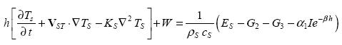
The model is based in the equation of conservation of thermal energy for the sea mixed layer:

............(1)

where: h(m) is the mixed layer thickness; T_S(°K) is the SST; V_ST (ms^–1), the horizontal velocity in the ocean mixed layer; , the two–dimensional gradient operator; K_S(m²s^–1), the constant horizontal exchange coefficient; W(°Kms^–1), the rate of cooling in the mixed layer due to turbulent vertical penetration of colder water from the thermocline (entrainment); E_S(Wm^–2), the rate at which energy is added by short–wave and long–wave radiation; G₂(Wm^–2), the rate at which the sensible heat is lost to the atmosphere by turbulent transport; G₃(Wm^–2), the rate at which the heat is lost due to evaporation; ₁Ie^–βh (Wm^–2), the penetrative solar radiation; and β=0.1 m^–1 the solar extinction coefficient (Alexander and Kim, 1976). The water density ps and the specific heat ρ_S are considered constant and equal to 1.035x10³ kgm^–3 and 4186.0 Jkg^–1 °K^–1 respectively.

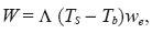
The entrainment term W(°Kms^–1) in equation (1) can be expressed as:

............................................................(2)

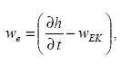
where w_e (ms^–1), is the entrainment velocity, which following Alexander (1992) is associated with the mixed layer deepening δh/δt modified by the Ekman pumping velocity w_EK(ms^–1), and is given by:

.............................................................(3)

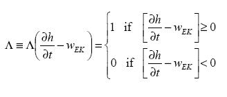
In equation (2) is the Heaviside function defined as:

.......................(4)

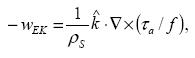
In equation (2), T_b(°K) is the sea water temperature below the mixed layer and the Ekman pumping velocity w_EK(ms^–1) is given by:

.................................................(5)

where is the vertical unit vector positive downward; (Nm^–2), the surface wind stress vector; and f=2Ωsinφ is the Coriolis parameter; Ω, the angular velocity of the Earth, and φ, the latitude.

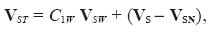
For the horizontal ocean currents V_ST(ms^–1) in the mixed layer in according with Adem (1970), we shall assume that:

.............................................(6)

where C_1w is an empirical coefficient, we are using C_1w=0.235 which assumes that the currents in the Gulf of México have a vertical profile in the frictional layer that is similar to the pure drift current; V_SW is the horizontal velocity of the normal seasonal surface ocean current, which is prescribed in the model using observed values. (Normal is used for monthly or seasonal longterm mean values). V_S is the horizontal velocity of the pure drift ocean current and V_SN its corresponding normal value.

The zonal and meridional components of V_S(ms^–1) are given (Adem 1970; Mendoza et al. 1994) by:

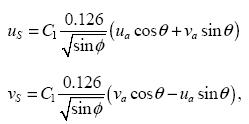
where u_S and v_S are the west–east and south–north components of the resultant pure drift current in the layer of depth h, respectively; and u_a and v_a are the west–east and south–north components of the surface wind, respectively.

The range of values of θ and C₁ are arbitrarily limited to:

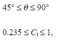
we have assigned θ=90° and C₁=0.235, which means that the resultant pure drift current is directed 90° to the right of the surface wind velocity, in concordance with the imposed surface stress and Ekman pumping velocity.

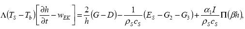
The equation of the model that represents a balance between mechanical energy and thermal energy, where the entrainment of cold water is determined according to Kraus and Turner (1967), is:

.......(7)

where G is the turbulent kinetic energy input from the wind, D is the dissipation within the layer, and Π(βh) is the solar penetration function, which is unity for complete penetration and zero for complete absorption. On the left side of equation (7), the first term represents the rate of work needed to lift and mix the more dense entrained water. On the right side, the first term represents the difference between the rate of generation and dissipation of turbulent kinetic energy produced by the wind, and the second and third terms represent the rate of potential energy change produced by the net heating and the penetration of solar radiation in the mixed layer.

The solar penetration function in equation (7) is given (Alexander and Kim, 1976) by:

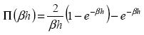...............................................(8)

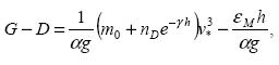
The difference between the rate of generation and dissipation of turbulent kinetic energy is given by:

....................................(9)

where =2.1 x 10^–4 °K^–1 is the thermal expansion coefficient of sea water; g = 9.8 ms^–2, the acceleration of gravity; m₀=1.25, an empirical parameter which was obtained from experimental results (Kato and Phillips, 1969); n_D=1.25 and =0.05 m^–1 parameters of dissipation; v_*, the frictional velocity related to the magnitude of the surface wind stress given by 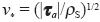; ε_M, the parameter of background dissipation, which exists even in the absence of wind stress, where ε_M= 2.0x10^–8 m²s^–3 for spring, ε_M=3.2x10^–8 m²s^–3 for summer and ε_M=0 for fall and winter.

For the magnitude of the surface wind stress (Nm^–2), we use the bulk formulas (Isemer and Hasse, 1987):

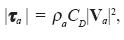...............................................................(10)

where and are the surface air density and the surface wind speed, respectively; and C_D, the atmospheric drag coefficient.

The west–east and south–north components of the wind stress vector are given, respectively, by:

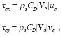...............................................................(11)

where u_a and v_a are the west–east and south–north components of the surface wind vector, respectively.

The rate at which the energy is added by short–wave and long–wave radiation at the sea surface (E_S) is computed as Budyko (1974) by:

..(12)

where δ= 0.96 is the emissivity of the sea surface; σ=8215x10^–14 calcm^–2 °K^–4min^–1 the Stefan–Boltzmann constant; T_a(°K), the ship–deck air temperature; U(%), the ship–deck air relative humidity; e_S(T_a), the saturation vapor pressure in hPa at the ship–deck air temperature; ε, the fractional amount of cloudiness; c=0.65, a cloud cover coefficient; and ₁I, the surface solar radiation, which is given by the Berliand–Budyko equation (Budyko, 1974):

............................(13)

where (Q + q)₀ is the total solar radiation received by the surface with clear sky; _S, the albedo of the sea surface; a and b are coefficients, where a is a function of the latitude and b is a constant equal to 0.38. For the Gulf of Mexico, we use a=0.35, which corresponds to 25 °N.

The heating functions G₂ and G₃ are given by the following formulae (Mendoza et al., 1997):

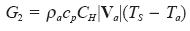..................................................(14)

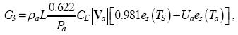....................(15)

where c_p=1.004 Jkg^–1K^–1 is the specific heat of air at constant pressure; L=2.44 x10⁶ Jkg^–1, the latent heat of vaporization that is considered constant; P_a, the sea level pressure; C_H and C_E, the vertical turbulent transport coefficients of the sensible and latent heat, respectively. The coefficients, C_D, C_H and C_E are determined as functions of the Richardson number R_i following Huang (1978). The saturation vapor pressure is computed using the equation proposed by Adem (1967).

 

2.1 A simple model for the cyclonic vortex

The wind speed profiles in the boundary layer of hurricanes Hilda and Gilbert can be described, in a first approach, by a function depending on the radius of the hurricane, as:

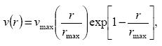.........................................(16)

where r (km) is the radius of the hurricane; r_max, the radius of the hurricane at which the tangential velocity is maximum; v(ms^–1), the tangential velocity; and v_max, the maximum tangential velocity at r= r_max. The position of the vortex and the values of the parameters r_max and v_max, are updated each 6 hours in agreement with the weather data of the hurricane. In Figure 3, we show the graph of the tangential velocity versus radius for the characteristic data of hurricane Hilda, when it was located in the center of the Gulf of México (24.72° N, 269.68° E), with a maximum tangential velocity of 68 ms^-1 and a radius of maximum tangential velocity of 40 km corresponding to the mature stage of this hurricane.

 

3. The integration method

Equations (1) and (7) were applied to time–average of one month and integrated in a uniform grid over the Gulf of México, the northwest Caribbean Sea and the Atlantic Ocean region contiguous to Florida. The time integration for equation (1) is explicit (Euler's method) and for equation (7) we use a backward implicit time finite differences scheme. We obtain for equation (1):

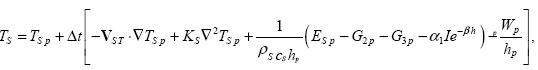.....(17)

and for equation (7):

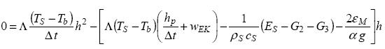
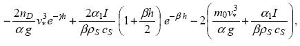...........................(18)

where we had used (8) and (9) in (7) to obtain equation (18) and where Δt is a time–step of 15 minutes. The subindex–p indicates that T_S and h have taken values of the previous time–step.

We compute h from equation (18) using the successive approximation method of Newton (Carnahan et al., 1969).

With T_S computed in the first time–step from equation (17), we compute h from equation (18) taking =1, which is applied if the first condition in (4) is satisfied. In this way, we obtained T_S and h for the first time–step. However, if the second condition in (4) is satisfied, then we compute h now specifying =0 in equation (18).

For the second time–step, we take as initial condition T_S and h, from the first time–step. The process is continued until completing the whole track of the hurricane.

For the spatial derivatives in equation (17), we used centered differences with a regular grid of 25 km, where the horizontal transport of heat by ocean currents and by turbulent eddies are taken as zero at the points in the closed boundaries (coasts). At the points in the open boundaries (in the Caribbean Sea and the Atlantic Ocean region contiguous to Florida), we assume that the horizontal transport of heat by turbulent eddies is negligible in comparison with the horizontal transport by ocean currents. For the horizontal transport of heat by ocean currents in the open boundaries, we compute the term using observed average values for the surface ocean currents and the sea surface temperatures.

 

3.1 Input–data

For the horizontal velocity vector of the surface ocean currents (V_SW), we use data for fall season derived from maps of the Mariano Global Surface Velocity Analysis (web site at http://oceancurrents.miami.edu/atlantic/loop–current.html).

For the zonal (u_a) and meridional (v_a) components of the surface wind we used the parameterization given by formula (16), and for the surface air temperature T_a, and the surface relative humidity U_a, we used the climate monthly values for September from NOAA–CIRES, Climate Diagnostic Center of Boulder Colorado (Web site at http://www.cdc.noaa.gov/). Seasonal values of the fractional amount of cloudiness ε, and the albedo of the sea surface _s, were obtained from data files used in Adem's thermodynamic climate model (Adem, 1965). For the temperature T_b, we used the sea water temperature at 61 m of depth from Robinson (1973). This value is approximately the average temperature of the thermocline, according to the profiles obtained from the analysis of temperature carried out by Robinson (1973) at 30.5, 61, 91.5, 122 and 150 meters of depth in the central part of the Gulf of México.

 

4. Results

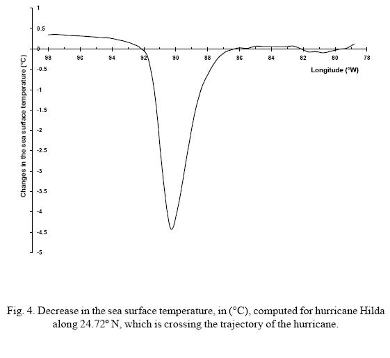
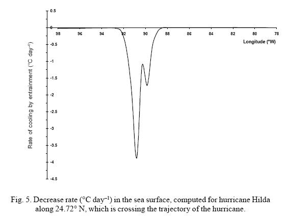
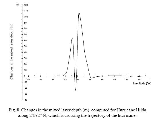
We computed the changes in the SST and the mixed layer depth with respect to the observed conditions of September in the Gulf of México produced by hurricane Hilda, when its axially–symmetric vortex had a maximum tangential velocity of 68 ms^–1 and its radius of maximum tangential velocity was 40 km. In the following figures, the left side indicates the west side of the path of the storm. The decrement in SST produced by this vortex along 24.72° N, which is crossing the trajectory of the hurricane, was approximately 4.5 °C in the center of the hurricane (Fig. 4). This contribution to the cooling is due mainly to the vertical turbulent water transport through the thermocline or entrainment, while to the left of center of the hurricane, the cooling rate is up 3.8 °Cday^–1 and to the right of 1.7 °Cday^–1 (Fig. 5). The balance of short and long wave radiation and the vertical turbulent transport of sensible and latent heat produces a return to the climate condition of September, due to heating rate in the center of the hurricane of 0.22, 0.13 and 0.07 °Cday^–1, respectively (Fig. 6). This "return to normal" effect is produced in a more important way by the horizontal turbulent transport of sensible heat associated with an "Austauch" coefficient of 3.0x10⁷ cm²s^–1 ', which produces a heating rate of 0.65 °Cday^–1 (Fig.7); however, the advection of heat by horizontal drift currents produced by the surface wind from hurricane, has a less effect over the change in the SST than the horizontal turbulent transport of sensible heat. The corresponding changes in the mixed layer depth (Fig. 8), indicate a deepening of 105 m to the east and 65 m to the west of the hurricane. At the center, the thermocline is lifted by 25 m with respect to the climatic condition. These predicted changes show qualitative agreement with the observations of Leipper (1967) that are shown in Figure 9, where a density anomaly band from 24.0 to 24.5, expressed as Sigma–t surfaces, rises in the center of the storm, which is shaded in the figure.

The entrainment velocity w_e, the Ekman pumping velocity w_EK and the mixed layer deepening, computed from the equation are shown in Figure 10. Whereas the most important contribution in the center of the hurricane is due to the Ekman pumping velocity (w_EK<0), the contribution by the mixed layer deepening () is practically zero. Outside of the center of the storm, the term >0 has an important contribution to the entrainment velocity that is only slightly reduced by the term w_EK>0.

The total cooling and the sinking of the thermocline computed by the model for hurricane Hilda during the crossing of the Gulf of México and its impact on the Louisiana coasts, are shown in Figure 11a and Figure 12, respectively. Comparison of Figure 11a with Figure 11b, shows a maximum decrease of 5 °C in the SST near 23.8° N, 89.5° W, while Leipper's observations indicate 1 °C. Also, the maximum decrease in the SST of 6 °C in Leipper's data near 25° N, 92° W, is underestimated by the model which indicate a decrease of 1 °C. This disagreement is probably due to the idealized axially–symmetric cyclonic vortex used in the model.

The total cooling and sinking of the thermocline computed by the model for hurricane Gilbert is shown in Figures 13a and 14, respectively, when it reaches the coast of Tamaulipas with intense winds (56 ms^–1), and produces a pronounced sinking of the thermocline and behind a wake of rising of the thermocline, which gives as result a pattern in the mixed layer depth similar to the one computed by the model for hurricane Hilda. Comparison of the figures 13a and 13b shows qualitative agreement with the observed cooling due to hurricane Gilbert.

 

5. Concluding remarks

We have studied the effects on SST due to the surface wind associated to axially–symmetric cyclonic vortex, characterized by two parameters: the maximum tangential velocity and the radius at which this velocity is reached; we have used characteristic values for these two parameters that correspond to hurricanes Hilda and Gilbert. Air temperature and humidity in sea surface, as well as cloudiness, are taken as climatic data and they are prescribed using the normal values for September month.

1. The simulations indicate that hurricanes produce a cooling in the sea surface of several Celsius degrees and a deepening of the thermocline of several tens of meters. Both processes are due mainly to the vertical turbulent transport of water through the thermocline (entrainment), these results are in agreement with the observations.

2. The most important contribution to the cooling takes place in the center of the hurricane and is due to the Ekman pumping velocity, whereas the contribution due to the mixed layer deepening () is practically zero. Out of the center of the storm, the deepening of the thermocline ( >0) has an important contribution in the cooling of the mixed layer.

3. The sensible and latent heat fluxes and the net radiation produce a heating rate in the sea surface of aproximately 0.15 °C day^–1, in comparison with the entrainment which produces a cooling of near of 4.0 °C day^–1. The results show that intense cooling of the sea surface produced by the hurricane reduces the sensible and latent heat fluxes to the atmosphere, which possibly moderates the intensity of the storm when the atmospheric instability is being reduced and there is not enough provision of heat from the ocean, as Black and Willoughby (1992) have mentioned.

4. The horizontal turbulent transport of heat associated to an "Austausch" coefficient, produces a heating greater than the produced by the net radiation and the sensible and latent heat fluxes, since the horizontal turbulent transport reaches 0.7 °Cday^–1 in the center of the hurricane Hilda, compared with approximately 0.2 °Cday^–1 produced by the heating functions. This heating rate induces a return to the normal or climate condition in the sea surface temperature, which was imposed as initial condition in the model.

5. The horizontal transport by the drift currents in the mixed layer is directed outward the center of the hurricane Hilda (90° to the right of the wind) and produces a negligible cooling compared with that produced by Ekman pumping.

In future works we will increase the density of the grid and will incorporate anomalous conditions in the cloudiness, air temperature and air humidity on the sea surface associated with the hurricane, which surely will modify the results as regards to contribution of the net radiation and the sensible and latent heat fluxes.

 

Acknowledgements

This work was supported by PAPIIT Project No. IN108705–2 (Programa de Apoyo a Proyectos de Investigación e Innovación Tecnológica. Universidad Nacional Autónoma de México). We are indebted to Berta Oda and Rodolfo Meza for the computational technical support.

 

References

Adem J., 1965. Experiments aiming at monthly and seasonal numerical weather prediction. Mon. Wea. Rev. 93, 495–503.        [ Links ]

Adem J., 1967. Parameterization of atmospheric humidity using cloudiness and temperature. Mon. Wea. Rev. 95, 83–88.        [ Links ]

Adem J., 1970. On the prediction of mean monthly ocean temperature. Tellus, 22, 410–430.        [ Links ]

Alexander M. A., 1992. Midlatitude atmosphere–ocean interaction during El Niño. Part I: The North Pacific Ocean. J. Climate 5, 944–958.        [ Links ]

Alexander R. C. and Jeong–Woo Kim, 1976. Diagnostic model study of mixed–layer depths in the summer North Pacific. J. Phys. Ocean. 6, 293–298.        [ Links ]

Black M. L. and H. L. Willoughby, 1992. The concentric eyewall of hurricane Gilbert. Mon. Wea. Rev. 120, 947–957.        [ Links ]

Budyko M. I., 1974. Climate and life. International Geophysics Series, 18, Academic Press, New York. 508 p.        [ Links ]

Carnahan B., H. A. Luther and J. O. Wilkes, 1969. Applied numerical methods. Wiley & Sons, 604 p.        [ Links ]

Fisher E. L., 1958. Hurricane and the sea–surface temperature field. J. Meteor. 15, 328–333.        [ Links ]

Huang J. C. K., 1978. Numerical simulation studies of oceanic anomalies in the North Pacific Basin, I. The ocean model and the long–term mean state. J. Phys. Ocean. 8, 755–778.        [ Links ]

Isemer H. J. and L. Hasse, 1987. The Bunker Climatic Atlas of the North Atlantic Ocean, Vol. 2. Air–Sea Interactions. Springer–Verlag, Berlin, 252 p.        [ Links ]

Kato H. and O. M. Phillips, 1969. On the penetration of a turbulent layer into a stratified fluid. J. Fluid Mech. 37, 643–655.        [ Links ]

Kraus E. B. and J. S. Turner, 1967. A one–dimensional model of the seasonal thermocline, II. The general theory and its consequences. Tellus 19, 98–106.        [ Links ]

Leipper D. F., 1967. Observed ocean conditions and hurricane Hilda, 1964. J. Atmos. Sci. 24, 182–196.        [ Links ]

Mendoza V. M., E. E. Villanueva and J. Adem, 1997. Numerical experiments on the prediction of the sea surface temperature anomalies in the Gulf of México. J. Mar. System. 13, 83–99.        [ Links ]

Mendoza V. M., E. E. Villanueva and J. Adem, 2005. On the annual cycle of the sea surface temperature and the mixed layer depth in the Gulf of México. Atmósfera, 18, 127–148.        [ Links ]

Peabody L. and A. F. Amos, 1989. 1988 Hurricane Gilbert's effect on sea–surface temperature. Mariners Weather Log. NOAA 33, 8–15.        [ Links ]

Robinson M. K., 1973. Atlas of monthly mean sea surface and subsurface temperature and depth of the top of the thermocline Gulf of México and Caribbean Sea. Scripps Inst. Ocean., Univ. California, San Diego, SIO Ref. 73–8.        [ Links ]

Shay L. K., P. G. Black, A. J. Mariano, J. D. Hawkins and R. L. Elsberry, 1992. Upper ocean response to hurricane Gilbert. J. Geo. Res. 97, 20227–20243.        [ Links ]