Barnes objective analysis scheme of daily rainfall over
Maharashtra (India) on a mesoscale grid

 

S. K. SINHA, S. G. NARKHEDKAR
Indian Institute of Tropical Meteorology, Dr. Homi Bhabha Road, Pashan, Pune – 411008, India
Corresponding author: S. K. Sinha; email: sinha@tropmet.res.in

A. K. MITRA
NCMRWF, DST, A–50, Institutional Area, Sector – 62, NOIDA, UP, 201 307, India
Email: akm_delhi@yahoo.com

 

Received April 4, 2005; accepted December 9, 2005

 

RESUMEN

En este trabajo se describe un análisis objetivo de la precipitación diaria sobre Maharashtra (India) por medio del peso de la función de la distancia en una red de mesoescala. Para interpolar en la red regular los datos de precipitación diaria distribuidos irregularmente se aplica el esquema de Barnes. La resolución espacial de los arreglos interpolados es de 0.25 grados de latitud por 0.25 grados de longitud. En este estudio se emplean algunas restricciones determinadas objetivamente: (i) los pesos se determinan como una función del espaciamiento de los datos, (ii) para lograr la convergencia de los valores analizados se realizan dos pasos por los datos, (iii) el espaciamiento de la red se determina objetivamente por el espaciamiento de los datos. Para este estudio se escogió el caso de una depresión monzónica típica con movimiento hacia el oeste durante la temporada de monzones de 1994. Se realizaron análisis objetivos de seis días (16 a 21 de agosto de 1994) utilizando la escala de longitud variable de dos pasos (V2P) y la escala de longitud fija de dos pasos (F2P) del esquema de Barnes. Se consideró una escala de longitud de 80 km para el paso externo y de 40 km para el paso interno. Los análisis mostraron una mejora moderada del esquema V2P sobre el F2P. La tendencia del análisis basado en V2P es 2 % menor que la del análisis basado en F2P.

 

ABSTRACT

An objective analysis of daily rainfall over Maharashtra (India) by distance weighting function on a mesoscale grid is described. The Barnes scheme is applied to interpolate irregularly distributed daily rainfall data on to a regular grid. The spatial resolution of the interpolated arrays is 0.25 degrees of latitude by 0.25 degrees of longitude. Some objectively determined constraints are employed in this study: (i) weights are determined as a function of data spacing, (ii) in order to achieve convergence of the analyzed values, two passes through the data are considered, (iii) grid spacing is objectively determined from the data spacing. The case of a typical westward moving monsoon depression during the 1994 monsoon season is chosen for this study. Objective analyses of six days (16 to 21 August 1994) have been carried out using variable length scale two pass (V2P) and fixed length scale two pass (F2P) Barnes scheme. A length scale of 80 km for the outer pass and 40 km for the inner pass are considered. Analyses show moderate improvement of V2P scheme over F2P scheme. The bias of the analysis based on V2P is 2% lower than that of analysis based on F2P.

Key words: Barnes scheme, mesoscale analysis, rainfall, monsoon depression.

 

1. Introduction

The Indian community generally regards rainfall as the most important meteorological parameter affecting its economic and social activities. Rainfall observations are needed to support a range of services extending from the real time monitoring and prediction of flood events to climatological studies of drought. For a wide range of applications, rainfall measurements over India are interpolated or extrapolated to ungauged locations where the information is desired but not measured. Numerical interpolation of irregularly distributed data to a regular N–dimensional array is usually called "objective analysis".

The existing observational network and synoptic methods of forecasting cannot predict mesoscale events except in very general terms. The meteorological data available on the Global Telecommunication System (GTS) and at the India Meteorological Department (IMD), New Delhi, raingauge data primarily cater to synoptic analysis and forecasting. These data do not have the required resolution in space and time to resolve and define mesoscale systems. There is an increasing demand for high resolution mesoscale weather information from different sectors like aviation, air pollution, agro–meteorology and hydrology. Mesoscale meteorology is of special importance as local severe weather events cause extensive damage to property and life. Lack of data on the mesoscale is one of the primary reasons for the poor understanding of mesoscale phenomena over the Indian region. Objectively analyzed data prepared by the National Centre for Medium Range Weather Forecasting (NCMRWF), New Delhi and IMD are of 1.5° Lat./Long. resolution, which is rather coarse for mesoscale NWP models having a resolution of 10 to 50 km. (0.1 to 0.5° Lat./Long.).

Mesoscale analysis is an important prerequisite for mesoscale research and modelling work. It has evolved into a specialized activity involving data acquisition, quality control checks, background first guess from the model, data ingest and assimilation. As of today, objective gridded analysis of mesoscale data is not available over the Indian region. Thus there is an urgent need to start work in developing a mesoscale analysis system. Our aim is to prepare a high resolution rainfall data over data rich regions. In this context we have tried to develop an objective analysis scheme of daily rainfall on a mesoscale grid. Raddatz (1987) examined the spatial representativeness of point rainfall measurements for Winnipeg (Canada) for two accumulation periods –one day and one month. Bussieres and Hogg (1989) made objective analysis of daily rainfall on a mesoscale grid using four different types of objective analysis schemes and compared the merits and demerits of different analysis techniques. Mitra et al. (1997) analyzed daily rainfall using the Cressman (1959) scheme over the Indian monsoon region by combining daily raingauge observations with the daily rainfall derived from INSAT IR radiances. The present study describes the details of the daily rainfall analysis on a mesoscale grid over the Maharashtra (India) region.

 

2. Synoptic condition and data

2.1.  Synoptic condition

Monsoon depression is very important so far as the distribution of rainfall in space and time over the region of its influence is concerned. Generally, 24 h accumulated rainfall is 10–20 cm and isolated falls can exceed 30 cm in 24 hours. On any particular morning heavy rainfall exceeding 7.5 cm extends to about 500 km ahead and 500 km to the rear of the depression centre and this area has a width of 400 km lying entirely to south of the track. The preferential rainfall is in the SW sector. Contribution of total depression associated rainfall is 11 to 16% in the left sector along the track (Mooley, 1973). During the summer monsoon short duration rainfall fluctuations are mainly due to westward passage of depressions, fluctuations in the intensity, location of the monsoon trough, and the low level westerly jet stream over the Arabian Sea. On an average, two to three monsoon depressions are observed per month during the monsoon period. The months of July and August experience the high frequency of these depressions. These systems have horizontal dimensions of around 500 km and their usual life span is about a week (Das, 1986). For Indian region, the standard deviation and the coefficient of variability for annual, summer monsoon (June to September total) and monthly rainfall are reported in tabular form and/or charts by Rao et al. (1971) and the IMD (1981). A general result in these reports is that rainfall amount and its relative variability are inversely related.

Daily rainfall analysis for a six day period starting from August 16, 1994 was carried out. This period was a very active phase of the monsoon, which caused heavy rainfall associated with the monsoon trough and also along the west coast of India. On 17 August a monsoon depression formed over the northwest of the Bay of Bengal and intensified into a deep depression on 18 August. Subsequently it moved in a northwesterly direction and lay over the northwestern part of the country on 20 August. It weakened into a low–pressure area by 21 August.

 

2.2.  Rainfall data

The domain of our analysis extends from 72°E to 83°E longitude and 15°N to 23°N latitude, cast on a fine mesh of 0.25° by 0.25° latitude/longitude grid. This particular domain covers all Maharashtra. The 24 hours' accumulated (valid at 03UTC) rainfall values from IMD raingauge observations coming through the GTS were collected. The GTS rainfall data over Maharashtra were supplemented by additional rainfall data obtained from the Agriculture Department of the Government of Maharashtra. Figure 1a shows the distribution of about 267 raingauge observations on a typical day. Latitudes and longitudes of different rainfall stations over Maharashtra are given in Table 1. Sub–division wise climatological normal rainfall values based on 1871–2003 over India for the monsoon season (June–September) have been given in the Table 2 and the locations of different sub–division of India are shown in Figure 1b. This will help to understand the characteristics of rainfall over Indian region.

 

3. Methodology

Barnes (1964, 1973) proposed an analysis scheme, which has probably replaced the Cressman analysis scheme (1959). The Cressman scheme corrects the background grid point values by a linear combination of residuals between predicted and observed values. These residuals are then weighted according to their distances from the grid point. The background field at each grid point is successively adjusted on the basis of nearby observations in a series of scans (usually three to four) through the data. The cutoff radius C_R(the radius of the circle containing the observations which influence the correction) is reduced on successive scans in order to build smaller scale information into the analyses where data density supports it. Cressman (1959) and Barnes (1973) objective analysis schemes are both weighted average techniques. One important difference is the choice of cutoff radius C_R. Cressman weights do not approach zero asymptotically with increasing distance as they do in the Barnes technique, but instead abruptly become zero at distance equal to C_R. This aspect of the Cressman scheme causes a serious problem when the data distribution is not uniform. The Barnes technique has gained wide importance in mesoscale analysis (e.g. Doswell, 1977; Maddox, 1980; Koch and McCarthy, 1982). This analysis produces a rainfall field on a regular grid from irregularly distributed observed rainfall stations. The rainfall estimated at a grid point "g" is a weighted average of surrounding observations, which are weighted according to the distance from the grid point. Achtemeier (1987) used a successive correction method so that an estimate of the rainfall fields is made on the first pass (iteration) and refined on successive passes. Inner passes, which yield incremental changes to the initial rainfall field, use shorter length scales so that relatively greater weight is assigned to observations close to an analysis grid point.

The analysis is performed using Barnes two pass successive correction system (Barnes, 1973; Koch et al., 1983). If a variable S(x_m, y_m) is observed at a location designated by m, then the first pass analysis at a grid point "g" is described by:

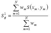............................................(1)

where the weight applied to the m^th observation is given by:

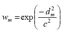....................................................(2)

The length scale c controls the rate of fall–off of the weighting function. Since the weight approaches zero asymptotically, there is no need to specify a radius of influence. However, the number of observations N should be chosen large enough so that the observations far away from the grid point receive a small weight. c exerts control over the filtering properties of the analysis.

The analysis after the second pass is given by:

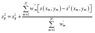........................(3)

where:

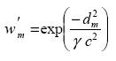..............................................................(4)

The analysis from the first pass provides a background field for the second pass. The weights produced by this function are in the range 0 to 1. is a numerical convergence parameter that controls the difference between the weights on the first and second passes, and lies between 0 and 1 (0 < < 1). Thus the weighting function has a steeper fall–off on the second pass in an attempt to build smaller scales into the analysis. Barnes (1964) objective analysis scheme without is convergent, but it requires several more passes to reach the same degree of convergence as compared to Barnes (1973) version with which requires only two passes through the data.

A simple bilinear interpolation between the values of S_g¹ at four surrounding grid points can be used to obtain an estimate for s¹(x_m, y_m) at each data location. If the average spacing of the data and the grid points is small compared to some wavelength , then the representation of that wavelength (response function) after the second pass is given by (Barnes, 1973):

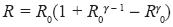.....................................................(5)

where 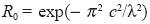is the response after the first pass. The response function R is the measure of the degree of convergence after a second pass through the data. The shape of the response curve is illustrated in Figure 2.

 

4. Results and discussion

4.1. Length scale and grid resolution

Objective determination of the analysis length scale (c) and grid resolution parameters (Δx) used in the analysis scheme is made from the method of Koch et al. (1983). The choice of both parameters is based on the average station separation, Δn and is given as:

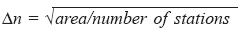
In the case of a daily rainfall network of about 267 stations over Maharashtra, Δn was found to be 0.6 degrees (approximately 60 km). Peterson and Middleton (1963) stated that a wave whose horizontal wavelength does not exceed at least 2Δn cannot be resolved, since five data points are required to describe a wave. Hence Δx should not be larger than half of Δn. Since a very small grid resolution may produce an unrealistic noisy derivative and if the derivative fields are to represent only resolvable features, the grid length should not be much smaller than Δn. Thus a constraint that Δn/3 < Δx < Δn/2 was imposed by Barnes in his interactive scheme. The analysis length scale (c) is fixed by the data spacing and is given as

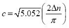
(Koch et al., 1983) which is roughly 80 km in this experiment, so that waves shorter than 2Δn are strongly filtered. Table 3 shows the values of different input parameters used in this experiment.

 

4.2. Analysis

Analyses of daily rainfall (16 to 21 August 1994) are carried out using a 2–pass (iteration) variable length scale Barnes scheme (here after referred to as V2P) and the standard 2–pass (iteration) fixed length scale Barnes (F2P) scheme. F2P and V2P are two ways of analysis. Pass here implies iteration, both (F2P and V2P) involve two passes. In the case of first pass (outer pass) =1.0 and in the second pass (inner pass) =0.3 are considered. F2P and V2P differ from each other in the sense that in F2P length scale (c) is fixed during both the iterations whereas in V2P length scale changes from first pass to second pass. Although analyses were made for six days, in Figure 3 the analyzed rainfall with V2P as well as F2P from 17 August to 20 August are shown, when the monsoon depression was passing in north–westerly direction from Bay of Bengal to North–West India. For 2–pass scheme, Koch et al. (1983) required to be in the range of 0.2 to 1.0, while Barnes (1973) suggested 0.2<<0.4. For the present study we have chosen length scale of 80 km for the outer pass (first iteration, =1.0) and the inner pass (second iteration) length scale of 40 km corresponding to =0.3 is chosen to add a reasonable amount of detail to the analyzed rainfall. On 17 August when the depression was over North–West Bay, analysis with F2P shows maximum rainfall of 40 mm whereas analysis with V2P shows maximum amount of 50 mm of rainfall over the same area. The contours are drawn at a regular interval of 10 mm. On 18 August when the system intensified into a deep depression, F2P shows a maximum amount of 30 mm rainfall at two places: one at 20° N, 74° E and other along the west coast. But the analysis with V2P shows 50 mm of rain at 20° N, 74° E and 30 mm of rain at three different places at a lower latitude along the west coast of Maharashtra. Around 20°N and 78.5°E, F2P shows 10 mm of rain whereas at the same place V2P shows 20 mm of rain. On 19 August the depression further moved landward. Comparing both the analyses (V2P and F2P), F2P shows rainfall maxima of 70 mm near 21 °N and 80°E, whereas V2P shows a maxima of 90 mm in the same region. In addition to this there are a number of regions along the west coast where V2P shows enhanced rainfall when compared to F2P (e.g. 20.5°N, 74.5°E; 16.5°N, 74.0°E). On 20 August (i.e. a day before the depression dissipated) F2P shows rainfall of about 20 mm at 20°N and 74°E, whereas V2P shows 40 mm of rain at the same place and at lower latitude along the west coast about 60 mm of rain is observed (V2P) compared to only 30 mm of rain (F2P). Thus it can be concluded that analyzed rainfall values with V2P are always higher than the F2P.

For the quantitative analysis of the rainfall root mean square (rms) errors for the six days are computed by comparing the analyzed rainfall against independent data not used in the analysis. This process is called cross validation approach and has been used widely dating back to Gandin (1963). That is, out of 267 observations 95% of data are used in the analysis and the verification is done on the remaining 5%. In the verification the analyzed values have been interpolated to the observation locations. The root mean squares (RMS) errors are generally between 8.15 to 16.58 mm for the V2P scheme, whereas for F2P they are in the range of 8.34 to 17.0 mm showing moderate improvement of the V2P scheme over F2P. As the distribution of rainfall amounts is positively skewed (non–normal) and the rainfall is highly variable, the rms error can give a misleading picture of rainfall analysis errors. This means a small number of large errors can unreasonably dominate rms statistics. Tapp et al. (1986) have shown that sometimes rms statistics on the cube root of rainfall amounts (which are less skewed) can sometimes give a better picture of the analysis error. Often a mean absolute error is a more reasonable measure of rainfall analysis accuracy than rms error. Table 4 shows the different types of errors and the standard deviations of rainfall on different days for the present study. It has been observed that when the standard deviation (SD) of the observed rainfall values is high, on those days the rms errors of the analyzed rain are also high. In many cases, bias is a more important measure of analysis accuracy since the total rainfall over an area, rather than the variation within the area, is often required from the analysis. Analyses based on V2P have been found to be more accurate than analyses using F2P. The bias of the analyses based on V2P is 2 % lower than that of analyses based on F2P.

In order to examine how the analysis changes with the variation of convergence parameter (), analysis with V1P (=1.0, c = 80 km, Fig. 4a) and V2P (=1.0, c=80 km; =0.3, c=40 km, Fig. 4b) are performed and displayed for 19 August. Figure 4b, which is for =0.3, shows a rainfall maxima of 80 mm over northeast Maharashtra. But analysis with =1.0 (Fig. 4a) shows maximum of 45 mm of rain over the same region. Also Figure 4a shows only 10 mm of rain over 20.5°N and 74.5°E whereas over the same region Figure 4b shows 40 mm of rain. At lower latitude along the west coast Figure 4a shows a maximum of 25 mm of rain but Figure 4b shows 40 to 60 mm of rain. Analysis of rainfall produced by V2P shows more number of maxima with lot of spatial variability, whereas analysis with V1P shows a very smooth distribution of rainfall.

Thus we find that analysis with V2P (=0.3) produces superior. Figure 5a shows the analysis of total of six days (16 to 21 August) rainfall with V2P. Analyzed rain for the same period with F2P is shown in Figure 5b. Maximum rainfall of about 160 mm (F2P) is seen along the west coast (Fig. 5b). But V2P (Fig. 5a) shows 150 to 200 mm of rain along the west coast. Contours are drawn at an interval of 20 mm. Average of daily rainfall (16 to 21 August 1994) at each grid point is computed for both the analyses V2P as well as F2P and following Mills et al. (1997) analysis of the absolute difference between the average daily rainfall fields in mm (V2P–F2P) is shown in Figure 6. Thus it can be concluded that V2P produced a better analysis.

 

5. Conclusions

No worthwhile mesoscale research and modelling work can be carried out without good quality of mesoscale data for the Indian region. The present study to analyze daily rainfall over Maharashtra is an effort in this direction. Daily rainfall analysis over Maharashtra has been produced using an interactive Barnes (1973) objective analysis scheme. Length scale and grid resolution are objectively determined from the average data spacing. Analyses with V2P as well as F2P Barnes scheme have been performed to examine the performance of the two schemes. Length scale of 80 km corresponding to =1.0 for the outer pass and length scale of 40 km for the inner pass with =0.3 are considered in this experiment.

It has been found that improvement in the analysis with V2P over F2P is moderate. Bias with V2P analysis is 2% less than F2P. Barnes (1994) has shown that analysis accuracy depends on the regularity of observation spacing. He found that in an objective analysis based on 77 randomly distributed observations mean absolute errors could be 40% higher than for an analysis based on 23 uniformly distributed observations. Thus for producing better quality of rainfall analysis we require more uniformly distributed rainfall observations. This scheme has the following advantages.

(i) There is no need to specify an influence radius

(ii) Two to three passes are required to reach convergence.

(iii) Background field (first guess) is not required. Therefore analysis can be performed without the use of a model.

Objective analyses for the six–day period were made using two passes (=1.0 and =0.3). Errors were computed by comparing the analyses with the observations using a cross validation technique. Mesoscale analysis involves assimilation of data from different sources and sensors. Plans are ahead to include satellite data to complement the existing raingauge data and the length scale used in this study can then be adjusted accordingly. Satellite data will also extend the analysis area over oceans and also over data sparse regions. Our main task is to combine optimally the raingauge data with data from other sources. Currently we are in the process of analyzing daily rainfall for longer periods over a larger region (whole India) and with number of different synoptic situations.

 

Acknowledgements

The authors are extremely grateful to Dr. G. B. Pant, Director, Indian Institute of Tropical Meteorology, Pune, for the necessary facilities. We are thankful to Shri P. Seetaramayya, Head, FRD for his encouragement. We also express our gratitude to the anonymous referees for the constructive comments and suggestions. Thanks are also due to India Meteorological Department and the Agriculture Department of Government of Maharashtra for providing us with the rainfall data. Last but not least we extend our thanks to Miss Anindita for her technical support.

 

References

Achtemeier G. L., 1987. On the concept of varying influence radii for a successive corrections objective analysis. Mon. Wea. Rev. 115, 1760–1771.        [ Links ]

Barnes S. L., 1964. A technique for maximizing details in a numerical weather map analysis. J. Appl. Meteorol. 3, 396–409.        [ Links ]

Barnes S. L., 1973. Mesoscale objective map analysis using weighted time–series observations. NOAA Tech. Memo. ERL NSSL–62, National Severe Storms Laboratory, Norman, OK 73069, 60 pp. [NTIS COM–73–10781].        [ Links ]

Barnes S. L., 1994. Applications of the Barnes objective analysis scheme. Part I: Effects of undersampling, wave position and station randomness. J. Atmos. Oceanic Tech. 11, 1433–1448.        [ Links ]

Bussieres N. and W. Hogg, 1989. The objective analysis of daily rainfall by distance weighting schemes on a mesoscale grid. Atmosphere–Ocean. 27, 521–541.        [ Links ]

Cressman G. P., 1959. An operational objective analysis system. Mon. Wea. Rev. 87, 367–374.        [ Links ]

Das P. K., 1986. Monsoons. WMO monograph No. 613, WMO, Geneva, 155 pp.        [ Links ]

Doswell C. A., 1977. Obtaining meteorologically significant surface divergence fields through the filtering property of objective analysis. Mon. Wea. Rev. 105, 885–892.        [ Links ]

Gandin L. S., 1963. Objective analysis of meteorological fields (in Russian). Israel Program for Scientific Translation. 242 pp.        [ Links ]

India Meteorological Department, 1981. Climatological atlas of India. Part I: Rainfall, New Delhi, 69 charts.        [ Links ]

Koch S. E. and J. McCarthy, 1982. The evolution of an Oklahoma dry line. Part II Boundary–layer forcing of mesoconvective systems. Mon. Wea. Rev. 39, 237–257.        [ Links ]

Koch S. E., M. desJardins and P. J. Kocin, 1983. An interactive Barnes objective map analysis scheme for use with satellite and conventional data. J. Clim. Appl. Meteorol. 22, 1487–1503.        [ Links ]

Maddox R. A., 1980. An objective technique for separating macroscale and mesoscale features in meteorological data.Mon. Wea. Rev. 108, 1108–1121.        [ Links ]

Mills G. A., G. Weymouth, D. Jones, E. E. Ebert, M. Manton, J. Lorkin and J. Kelly, 1997. A National objective daily rainfall analysis system. BMRC Techniques Development Report No. 1 30 pp.        [ Links ]

Mitra A. K., A. K. Bohra and D. Rajan, 1997. Daily rainfall analysis for Indian summer monsoon region. Int. J. Clim. 17, 1083–1092.        [ Links ]

Mooley D. A., 1973. Some aspects of Indian monsoon depressions and associated rainfall. Mon. Wea. Rev. 101, 271–280.        [ Links ]

Peterson D. P. and D. Middleton, 1963. On representative observations. Tellus 15, 387–405.        [ Links ]

Raddatz R. L., 1987. Mesoscale representativeness of rainfall measurements for Winnipeg. Atmosphere– Ocean, 25, 267–278.        [ Links ]

Rao K. N., C. J. George and V. P. Abhyankar, 1971. Nature of the frequency distribution of Indian rainfall (monsoon and annual). Rep. No. 168, India Meteorological Department, Pune, India.        [ Links ]