Characteristics of the surface layer above a row crop
in the presence of local advection

 

P. I. FIGUEROLA
Departamento de Ciencias de la Atmósfera y los Océanos,
Facultad de Ciencias Exactas y Naturales, Universidad de Buenos Aires,
Ciudad Universitaria 1428, Buenos Aires, Argentina
Corresponding author e–mail: figuerol@at.fcen.uba.ar

P. R. BERLINER
Blaustein Institute for Desert Research, Ben–Gurion University of the Negev,
Sede Boqer Campus, Israel

 

Received September 8, 2004; accepted December 6, 2005

 

RESUMEN

En algunas regiones áridas los campos cultivados no son contiguos y están rodeados por grandes áreas de suelo desnudo. Durante el verano, estación sin lluvia con alta radiación solar, la temperatura del suelo durante el día en las áreas desnudas y secas es mucho más alta que la del aire. El calor sensible generado sobre estas zonas puede ser advectado hacia los campos irrigados. Los cultivos son usualmente plantados en hileras y son irrigados por sistema de goteo, no mojando totalmente la superficie del suelo. El suelo desnudo y seco entre las hileras del cultivo alcanza altas temperaturas y lleva a una convección dentro del cultivo entre las hileras. La advección desde el área seca de los alrededores y la actividad convectiva dentro del cultivo entre el suelo desnudo afecta la capa arriba del cultivo. Se estudió la capa superficial encima de un cultivo irrigado de tomate plantado en el desierto del Negev, Israel. El cultivo fue plantado en hileras, irrigado por goteo y la distancia entre bordes y dos filas adyacentes era de 0.36 m al momento de realizar las mediciones. Los gradientes de temperatura y presión de vapor de agua fueron medidos a varias alturas arriba de la cobertura vegetal con un apartado de Bowen. El residuo de la ecuación de balance de energía fue usado como criterio para determinar la capa de equilibrio. Durante la mañana predominaron condiciones inestables y la capa interna de equilibrio estuvo entre Z/h ˜ 1.9 a 2.4. En algunas circunstancias, a las últimas horas de la mañana, el suelo desnudo entre las hileras alcanza temperaturas extremas altas y baja velocidad del viento siendo identificadas situaciones de convección libre. Durante estas horas, el residuo para las alturas Z/h ˜ 1.5 y 2.4 fue significativamente diferente de cero y fue evidente una extrema variabilidad para las capas Z/h = 3.2. La advección local ocurre después del mediodía, resultando en un aumento de la estabilidad en la capa más alta que se propagó hacia abajo. La capa de equilibrio estuvo entre Z/h ˜1.5 y 2.4. Los residuos fueron significativamente diferentes de cero para las capas más altas Z/h ˜ 2.7 a 3.2 durante este periodo. Los resultados indican que la profundidad y ubicación de la capa interna de equilibrio, encima del campo irrigado rodeado por áreas desérticas, responde a la velocidad del viento y la temperatura del suelo entre las hileras del cultivo. Para algunos intervalos, el cálculo de los flujos usando la aproximación de flujos gradientes no fue posible.

 

ABSTRACT

In some arid land, the irrigated fields are not contiguous and are surrounded by large patches of bare land. During the summer time and rainless season, the solar radiation flux is high and the surface temperature during daylight in the dry bare areas, is much higher than that of the air. The sensible heat generated over these areas may be advected to the irrigated fields. The crops are usually planted in rows and the irrigation systems used (trickle) do not wet the whole surface, the dry bare soil between the rows may develop high soil surface temperatures and lead to convective activity inside the canopy above the bare soil. Advection from the surrounding fields and convective activity inside the canopy affect the layer above the crop. We studied the surface layer above an irrigated tomato field planted in Israel's Negev desert. The crop was planted in rows, trickle irrigated and the distance between the outer edges of two adjacent rows was 0.36 m at the time of measurement. The gradients in temperature and water vapor pressure were obtained at various heights above the canopy using a Bowen ratio machine. The residual in the energy balance equation was used as a criterion to determine the equilibrium layer. During the morning, unstable conditions prevail, and the equilibrium layer was between Z/h ˜ 1.9 and 2.4. In some particular circumstances, in the late morning, the bare soil between the rows reached extremely high temperatures and during conditions with low wind speeds free convection was identified. During these hours the "residuals" of the energy budget to the heights Z/h= 1.5 and 2.4 were significantly different from zero and an extremely large variability was evident for the Z/h = 3.2 layer. Local advection took place during the afternoon resulting in an increase in the stability of the uppermost measured layer and propagated slowly downwards. The equilibrium layer was between Z/h ˜ 1.5 to 2.4. The residuals were significantly different from zero for the uppermost layers Z/h = 2.7 and 3.2 during these periods. Our findings suggest that the depth and location of the internal equilibrium layer above trickle irrigated row crop fields surrounded by dry bare areas, vary in response to wind speed and the temperature of the soil in between the rows of the crop. For some time intervals, the computation of fluxes using the conventional flux–gradient approach measurements was not possible

Keywords: Advection, row crop, convection.

 

1. Introduction

Evaporation of water is a key element in the regional water balance of semi–arid regions and its quantification is necessary in order to manage successfully the limited water resources of these areas. A convenient and well–established approach to achieve this goal is to estimate the flux density of latent heat within the surface layer that lies above the vegetated area (Monteith and Unsworth, 1990).

The spatial discontinuity is very pronounced in arid and semi–arid regions, where locally the crops are surrounded by dry land. When an air mass moves from a surface to one with different characteristics, the lower boundary conditions change abruptly and it must adjust to the new set of boundary conditions. Downwind of the new roughness, an internal boundary layer develops growing in height with downwind distance, whose properties have been affected by the new surface. The adjustment is not immediate throughout thickness of the air layer. Bradley (1968) and Mulhearn (1977), describing the downwind velocity profiles within the internal boundary layer, suggested that it might be described through a modified logarithmic law. Far downwind of the roughness change, a new equilibrium may be visualized so that the stress everywhere is constant. The region where has been achieved a new equilibrium with the new surface is often called the equilibrium layer and the logarithmic laws can be applied. This layer is the lowest region, about the lowest 10% of the internal boundary layer; it is supported as far as the roughness change (Kaimal and Finnigan, 1994).

Local advection is the situation in which the growing internal boundary layer is no deeper than the upstream surface layer, and shows the development of a deepening inversion layer in an existing unstable lapse profile, referred as an advective inversion. It is the classical agrometeorological circumstance of airflow from hot dry to cool irrigated pasture (Dyer and Crawford, 1965).

In our case of row crops that do not completely cover the soil, the lack of surface homogeneity introduces a complicating factor. Vorticular flow patterns appear when λ/h >> λ, where l is row spacing and h is crop height (Perrier et al., 1972). The roughness sublayer is the region at the bottom of the internal boundary layer, where the presence of the canopy impinges directly on the character of the turbulence. Further problems in applying the semi–logarithmic profile laws and their diabatic extensions could be encountered.

In arid and semi–arid areas, two factors increase the complexity of the soil–plant–atmosphere system: the influence of local advection and the high temperatures of the bare soil between the rows of the crop. The transport of energy in the horizontal plane is classified as being either regional or local. The former case describes situations in which the transport of sensible heat energy is the result of warm dry air masses on a synoptic scale or mesoscale (Prueger et al., 1996). The latter describes the local flow between two adjacent fields. An example of local advection is an irrigated field crop bordered by a large area of dry fallow land. This is a common feature of arid and semi–arid regions, as irrigated areas frequently occupy small patches of land that are surrounded by large bare areas. In this case, the horizontal advection of sensible heat increases the evaporation of water from the irrigated areas. Lee et al. (2004) describe the characteristic differences between local and regional advection.

High temperatures of the soil surface, the second complicating factor mentioned above, are the result of the fact that row crops in arid areas are usually watered using trickle irrigation, which results in the localized wetting along the rows of the crop. The bare areas in between the rows of the crop are dry and due to the high solar radiation, typical of these areas, the soil surface temperature may reach very high values and generate plumes of hot air. These plumes may therefore enhance the strong horizontal lack of homogeneity due to the structure of the crop.

Consequently, local advection would result in the lowering of the upper boundary of the internal boundary layer and its equilibrium layer, while the incomplete cover and the associated plumes from the bottom would lead to an increase in the height of the lower boundary. A description is presented in Figure 1.

The three most common micrometeorological methods used to estimate actual evapotranspiration above a crop are based on the Bowen ratio, the aerodynamic equation, and the Penman–Monteith equation (Brutsaert, 1982). The application of these methods requires horizontal advection to be negligible when compared to the magnitude of the vertical fluxes. In this case, the closure of the energy balance equation for an imaginary plane located above the canopy must be satisfied. The aerodynamic method has to be applied (Rana and Katerji, 2000) at heights that are larger compared to the roughness length and smaller compared to the boundary layer depth. To perform the routine estimation of fluxes, much care must be taken to analyze local advection under arid conditions (Prueger et al., 1996) and in plot without enough fetch. In mixed plant communities, hilly terrains and small plots these techniques cannot be used (Rana and Katerji, 2000).

The height where the energy closure is calculated may vary because it depends on the distance to the border of the field, humidity conditions of the soil, plant density and height, and also, the energetic and dynamic conditions of the flow field. An experiment was undertaken in order to estimate the height interval above a row crop over which fluxes could be computed using the conventional micrometeorological methods in the presence of advection, therefore the crop evapotranspiration can be estimated being of particular importance in arid zones.

 

2. Materials and methods

2.1 The area: general features

The Negev is located on the northern border of the planetary desert and is a continuation of the Egyptian desert. The rainfall near the coast is 100–150 mm and drops sharply towards the south. Prevailing pressure systems and their interaction with local land features establish the wind regime of any given place. Except for its extreme south, a land and sea breeze system affects most of the Negev. During the summer months, a semi–permanent low–pressure trough extends from the Persian Gulf to the northeastern Mediterranean, causing a general northwesterly flow over the entire country, modified by the sea breeze. During the summer the sea–land breeze produces a daytime westerly–northwesterly component over the northern and western Negev, becoming easterly southeasterly at night (Zangvil et al., 1991).

Kibbutz Mashabei–Sade, on whose fields the trial was carried out, is located about 60 km from the Mediterranean coast and 50 km south of the city of Beer–Sheva (32 °N, 34 °E), in the south of Israel. Data obtained from available records at a meteorological station at Mashash (5 km from the experimental field), indicate that during the summer wind directions at 10 m high are mainly from the north–northwest between 8:00h until 22:00h, becoming easterly during the night. The wind speeds are low during the morning and higher in the afternoon.

Field trial was carried out between 8 and 14 September 1999 on a commercial tomato field (330 x 220 m) at Kibbutz Mashabei–Sade. The field was surrounded on the west and south by fallow fields, on the north by a field planted with jojoba, and on the east by an olive grove. The distance between rows was 2 m. In Table I, the average distance between the outer edges of two adjacent canopy rows is presented, as well as the average height of the crop. The crop was trickle irrigated with brackish water (EC = 6 dSm^–1) every three days.

 

2.2. Data acquisition

The Bowen ratio machine was designed with a distance of 0.5 m between psychrometers, thus spanning a total height interval of 1.5 m. The machine was installed at various heights by shifting it on a pole, and the height was regularly changed throughout the measuring period (Table I). The lowest measuring height was 0.8 m, 0.2 m above the canopy.

Profiles of horizontal wind speed were measured using four three–cup anemometers (014A Med–One) set at the same measuring heights as the psychrometers in the Bowen ratio system. The outputs of all meteorological sensors were recorded with a Campbell CR23X data logger.

A four–level Bowen machine with six–aspirated thermocouple psychrometers was used for above–canopy measurements (three on each side). The positions of adjacent psychrometers were interchanged every five minutes during the 30 min. The data were stored every four minutes plus one–minute rest, obtaining four levels of measurement. A representation of the Bowen ratio machine is showed in Figure 2.

Copper–constant thermocouples were used as temperature sensors. The thermocouples (0.5 mm) were with a low frequency response and it was necessary to shield them. The psychrometers were lined with polyurethane boards and covered by aluminum foil, both on the inside and on the outside. Wind speed in the psychrometer duct close to the sensors was estimated at 4 ms^–1. Sensors from adjacent heights were wired differentially and measured differentially with a CR23X datalogger. Particular attention was paid to the proper functioning of the wet bulb. The wick was wetted using a Mariotte bottle located inside the psychrometer, downwind of the sensors, thus virtually eliminating the dangers of radiative heating of the water reservoir. The water supply system functioned satisfactorily even during events with very high temperatures and unusually low relative humidity (35 °C and 25%, respectively). The paired thermocouples were tested in the lab by measuring temperature differences when placed in a well–stirred water bath. Average differences in the order of 0.05 °C were registered. Pairs of psychrometers were tested in the lab and in the field. In both cases, the intakes of the two psychrometers were placed in one box with a hole in the distal end. The Bowen machine and the anemometers were tested at Wadi Mashash Experimental Farm at 10 km from the Institute. The experimental field soil is sandy loam and completely bared, the place is wide open without obstacles or trees near, only the lab is there. The Bowen machine was installed outside in the prevailing wind direction (N – NW). The pair of psychrometers was placed at the same level at each height (Fig. 2). Typical differences, ranging from 0.02 to 0.2 °C for dry and wet bulbs, respectively, were registered and could only be the result of slight construction differences. The anemometers were calibrated relative to each other by setting them up at the same height in the open field.

Canopy temperatures and the row–gap soil temperatures were measured with an infrared thermometer, IRT (Telatemp Model AG42) and each measurement was taken on the crop (T_ic) and on the bare soil surface (T_is). The IRT was held at 45° from the horizontal and aimed at the same predetermined points throughout the trial. Three readings were taken at each point and the average used.

Net radiation was measured at 2 m above the canopy (Q–7, Campbell Scientific) and soil heat flux was measured with two–heat flux plates (HFT–3, Campbell Scientific) buried at a depth of 2 cm in the soil, one midway between the rows and the other under the vegetation. The copper–constant thermocouples were placed one under the canopy and the bare soil, at a depth of a few millimeters (0.012m). Global radiation was available from routine data measured with an Eppley precision pyranometer at the Blaustein Institute for Desert Research (Ben–Gurion University of the Negev) located at 5 km.

 

2.2.1 Data

Measurements were carried out on the following days: 251 (8/9), 252 (9/9), 254 (11/9), 255 (12/9), 256 (13/9) and 257 (14/9). The crop was irrigated every third day, on days 254 and 257, irrigation started at 14:00 h. Typical diurnal changes of temperature profiles above the canopy are slightly unstable during the morning, are almost isothermal at noon, and show a weak inversion thereafter.

The predominant wind direction was from the NW and N. Wind gusts from the W or NE were observed usually before midday, when the average wind speed was low. After 13:00 h, the wind speed increased and generally blew across the rows from the NW with enough fetch. The daily maximum temperature and the minimum daily relative humidity were between 30 to 35 °C and 30 to 40%, respectively; as measured at the weather station located nearby. The soil surface temperature measured by infrared thermometer may reach 55 °C at noon.

 

2.3 Micrometeorology parameters

Stability conditions are defined using the gradient Richardson Number (Ri) (Thom, 1975):

...................................................(1)

where, θ_i, θ_j and u_i, u_j are respectively, the potential temperature (K) and wind speed (ms^–1); measured at heights z_i and z_j (m); g is the acceleration due to gravity (ms^–2) and θ is the average temperature within the height interval (K). While different criteria have been suggested for defining neutral stability, we adopted Thom's (1975) criterion of < 0.01. The Richardson number was estimated from the data measured at the highest and lowest levels (i = 4, j = 1, see Table I) and the computed Ri are presented in Figure 3a. The common feature is one of unstable conditions before noon and stable conditions in the afternoon. High wind speeds occur during the afternoon as result of the breeze, (Fig. 3b).

Several arguments have been put forward to explain the anomaly in flux–gradient relationships in the roughness sublayer, in terms of wake diffusion, horizontal inhomogeneity, vertical location of sources and sinks. It has also been argued that these anomalies could vanish by adjusting the zero–plane displacement height (d) (Hicks et. al., 1979). Garratt (1979) and Raupach (1979) rejected this argument.

We obtained the zero–plane displacement height (d) and the roughness length (z₀) using Robinson's (1962) approach. The approach employs a minimum of four levels of wind measurements to mathematically solve for d and z₀, using the accepted logarithmic wind profile under neutral condition. The sum of the squares of errors to be minimized:

....................................(2)

where the subscript i stands for the i–th level of wind speed. The equation is differentiated with respect to u_*, d and z₀ and equated to zero. This expression is essentially a linear function of d that can be solved numerically by simple bisection to within ± 1 mm of the solution.

The Robinson's (1968) approach was used by Kustas et al. (1989), who compared the sensible heat flux calculated using the flux–gradient theory and sonic anemometer, finding that z₀ and d will differ depending on whether the flow is generally across or along the rows. Schween et al. (1997) obtain d with this approach finding that friction velocity u_* (calculated from flux–gradient theory) fit the measured values very well. However, the sensible heat flux is estimated too low.

We analyzed only neutral conditions (Ri < 0.015) and the cases for which the average wind speed was below 1.5 ms^–1 were excluded. Results are presented in Table II. The wind data led only to few values for d and z₀. Seeing the table, in the highest layer the Ri values were > 0.015, except one case where the d value was 0.380 m, agreeing well with the average d value (= 0.383 m ± 0.05 m).

The ratio of both quantities to the height of the obstacles, h, was z₀/h ≈ 0.033 and d/h ≈ 0.63 when the canopy height was 0.61 m, this latter compares well with the ratio suggested by Thom (1975). From summary of Raupach et al. (1991) with a roughness density, λ, approximately 0.7 (Hebbar et al., 2004) z₀/h and d/h should be about 0.10 and 0.67, respectively. The lower z₀/h ≈ 0.03 observed instead of 0.10 could be due to the winds blow along the rows. We will show later the error analysis to friction velocity and the sensible heat flux in relation to d. In advance, we can say that the friction velocity error is no affected for d.

Elliot (1958) proposed an empirical formula for the internal boundary layer, δ_i:

..............................................................(3).

where z₀₂ is the roughness length after roughness change, x the distance from the border, fetch, and A₁ is a constant of proportionality and has a weak dependence on the strength of the roughness change: A₁=0.75+0.03 M, where M=ln(z₀₁)/ln(z₀₂) and z₀₁ is before roughness change. In agreement with Monteith and Unsworth (1990) we used the equation (3) with M = 0 as the minimum depth (M is negative in smooth–rough change).

Based on wind tunnel evidence the flux of momentum is constant in the lowest 10–15 % of the turbulent boundary layer (Bradley, 1968), the logarithmic wind profile would be expected to extend to a height δ_i' = 0.01δ_i often called the internal equilibrium layer (IEL). Jegede and Foken (1999) have demonstrated in his study that the expression δ_i' = 0.3x^0.5 can safely be used to determine the height of the internal equilibrium layer that is free of the influence of overlying the internal boundary layer. For our experiment it is δ_i' = 4.5 m with x = 230 m. We have not enough data at a higher altitude to confirm this.

The internal boundary layer depth was computed according to equation (3) being x the fetch equal to 230 m when the wind direction is from WNW and to 318 m when it is from NW (M = 0). The resulting boundary layer depth, δ_i is between 26.6 to 34.5 m, then the internal equilibrium layer, δ_i', is 2.6 m and 3.4 m from WNW and NW direction, respectively.

The review achieved by Kaimal and Finnigan (1994) of the experiments where the approach to local equilibrium, or more directly, the validity of the flux–gradient connection can be compared with fetch, suggests that eddy diffusivities should be used with the greatest caution at fetch x < 10δ_i.

 

3. Methodology and results

3.1. Profiles

We define the gradients of temperature and vapor pressure as:

.........................................................(4)

where is the value of the relevant entity (temperature or vapor pressure) on adjacent levels and Z_j the mean geometric height:( 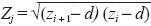) ofthe corresponding levels i(= 1, 2, 3). This gradient is first suggested by Panofsky (1965) and used by Paulson (1970).

 

3.1.1. The temperature profiles

In Figure 4 the temperature gradients at various heights (expressed as Z_j/h, with h the crop height) for days 251, 254 and 255 are presented, and the levels of measurements are detailed in Table I. For example, on day 251, the lowest level was at 1.5 m and the highest at 3.0 m. Graphs for the remaining three days were similar.

A typical example of the behaviour of the gradients is presented in Figure 4. The sign of the temperature gradient changes close to midday. The gradients were largest in the lowest layers and exhibited less change in the highest layers. The sign first changed in the highest layer, one hour thereafter in the intermediate layer (Z_j/h = 1.9), and two hours later in the lowest one. A similar behaviour was observed when the Bowen ratio machine was installed at different heights. The inversion temperature gradient in the afternoon was observed constant at the top (Fig. 4, Z_j/h = 3.9).

The development of an inversion layer is referred as an advective inversion, representing the circumstance of airflow blow from hot dry area to cool irrigated pasture (Dyer and Crawford, 1965).

Systematic measurements were not observed upwind, but data from a meteorology station outside showed that the air upwind temperature was usually higher (˜2 °C) than downwind and the temperature of the bare sandy soil can reach to 60 °C at noon. In some level above the boundary layer, the stable (inversion) temperature profile above the wet surface (downwind) lost connection with the surface, and it should follow with unstable temperature profile upwind.

Our results agree with Kroon and Bink (1996). They investigated the turbulent fluctuations in the internal boundary layer which forms in the wake of a dry to wet surface transition. They defined three periods with different thermal stability regimes: (1) morning with an unstable stratification up and downstream of the transition, (2) afternoon, when downstream of the transition the stratification changes from unstable to stable, while upstream the conditions remain unstable, (3) evening with stable stratification upstream and downstream.

 

3.1.2. The vapor pressure profiles

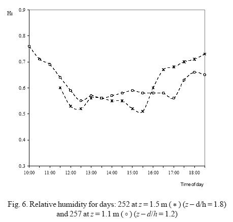
The vapor pressure gradient above an actively transpiring crop should diminish with height and this was observed everyday. Day 255 is presented as an example in Figure 5a (Z_j/h = 1, 1.9 and 2.7). When the tower was placed higher, for example, on day 252 (Fig. 5b), the gradient at Z_jh = 3 was larger than at Z_j/h = 2.2. This occurred after 14:00 h and it could be due to the influx of hot dry air.

In Figure 6, the relative humidity is presented for days 252 at z = 1.5 m (Z/h = 1.8) and 257 at 1.1m(Z/h= 1.2). In each case, there isa "plateau" in the relative humidity from 12:00 until 16:00 h (day 252) or 17:00 h (day 257) due to irrigation. A minimum relative humidity close to 30% (14:00 h) was measured at the meteorological station outside the field and this increased monotonically up to 80–90% at night. The "plateau" could not be observed.

Prueger et al. (1996) measured temperature and humidity profiles in a study around a well–watered alfalfa field surrounded by arid surfaces. Downwind the edge, they had shown that the profiles describe an inversion temperature and humidity decrease with height, the same case shown by us. Using eddy correlation, they found a negative heat sensible flux and a positive heat latent flux with height values (˜ 500 W m^–2). Stull (1988) says that under these conditions (negative heat sensible flux, positive heat latent flux and positive net radiation) an exceptional case of the oasis effect, due to the excess of evaporation from a well–irrigated surface, ocurrs. Summarizing, in our case, the wind speed is stronger during the afternoon, developing an inversion of temperature and a strong vapour pressure gradient over the irrigated tomato field.

 

3.2. The convective activity

Jacobs et al. (1994) showed that a decoupling between above–and within–canopy processes develops under conditions of low speed winds at night. Moreover, inside of the canopy, the relatively warm floor generates free convection cells. This argument can extend to those daylight hours during which low wind speed, high radiation prevail (late morning and midday) and high temperatures in the bare soil between the rows crop occurs, resulting in strongly unstable conditions inside the canopy. We observed that the temperature differences between the non–covered soil surface (T_is) and the air temperature measured at the lowest level above the canopy (T_is – T_a) are of the same order of magnitude as the differences between the former and the covered soil surface temperature, T_sc (under the plants), T_h = (T_is – T_sc). This fact supports the view that convective activity could take place during the previously defined time intervals.

Monteith and Unsworth (1990) use the ratio of the Grashof (Gr) to the Reynolds (Re) numbers (C₀=Gr/Re²) to identify the ranges of convection. The pure forced convection and pure free convection regimes occur when C₀<0.1 and C₀>16, respectively, and mixed convection occurs when 16<C₀< 0.1.

Raupach (1979), Jacobs et al. (1994) and Zelger et al. (1997) suggested that for the computation of Re within a canopy, the friction velocity u_* derived from above canopy wind speed profiles be a more convenient choice instead of the wind speed within the canopy. If the distribution of sources and sinks is determined by the dominant roughness structure (Ford, 1976; Raupach, 1979; Jacobs and Verhoef, 1997); δ could be identified, in our case, as the mean inter–row spacing and C₀ defined as:

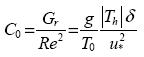.............................................................(5)

and δ is, in our case set, as 0.36 m, the average distance between the outer edges of two adjacent canopy rows during the measurement period. By definition, C₀ depends directly of T_h. The high valor's C₀ means that high soil temperature or low wind speed occurs. If both situations happen then it is a free convection case.

We evaluated the friction velocity, u_*,with the lowest level of wind speed observed. The diurnal variation of estimated values of C₀ (Eq. 5) for days 254, 255, 256 and 257 are presented in Figure 7. A few values with C₀>16 (free convection conditions) are evident during brief periods of extremely low wind speed, before 15:00 h. The lowest values of C₀(<0.1) were measured during the afternoon and coincide with the periods during which high wind speeds occurred. This is a common feature in the area during summer time due to the influence of the breeze. The error propagation to C₀(see 3.4.) is:

................................................................(6)

with C₀<1 it is dC₀/C₀<1, while if C₀>1 results that dC₀/C₀ increases as a potential function of C₀. The free convection case with C₀=100 results in a big error so that dC₀/C₀=8.

Another way to define convective activity from the bare soil between the rows crop was using the free convection velocity. This is: (7)

........................................................(7)

where is the kinematic heat flux at the soil surface, and T is the air temperature at the lower level.

An appropriate estimate (for scaling purposes) of the kinematic heat flux, at the bare soil surface, assuming negligible latent heat flux (a reasonable approximation in the case of a very dry surface), is:

...............................................(8)

where R_Ns and G_s are the net radiation and the heat soil flux at the floor over the bare soil. R_Ns was estimated from:

.............................(9)

where T_s is the soil surface temperature (as measured with an infrared thermometer), ε_s the emissivity of the soil (= 0.99), ε_a emissivity of air equal to 124(ε_a/T_a)^1/7 (Brutsaert, 1982), where T_a and ε_a are the temperature and the water vapor pressure of air observed at the upper level, a is the albedo (estimated from spot measurements as 0.3), and R_g the global radiation. The R_Ns computed by (9) slightly underestimates the actual flux density as long wave radiation emitted from the canopy, and short wave radiation scattered downwards by the canopy were not considered. The computed values of w_* are therefore slight underestimates as well. The value R_N is different at R_Ns because this latter has in consideration the bare soil temperature between the rows only.

Low wind speeds at canopy height (u(h) < 1 ms^–1) and w_* > u_*, are necessary conditions during nighttime for free convection to persist (Jacobs et al., 1994). During daytime these conditions will not be usually met, but a significant decrease of the horizontal wind velocity leads to a strongly reduced u_*, which coupled with larger values for the free convection scaling velocity w_* could result in conditions under which free convection could persist (Stull, 1988).

Figure 8 shows the values of w_* and u_* between 10:00 to 17:30 h. Values of w_*>>u_* occurred at 12:00, 13:30 h and 14:00 h during periods when extremely high soil surface temperature (T_is) were measured (43.6 °C, 52.7 °C and 53.9 °C, respectively). The cases for which w_*< u_* coincide with values of C₀ less than 16 indicated that mixed or forced convection conditions prevailed. Data of day 257, between 11:00 and 13:00 h were lost due to the stack of anemometer when low wind speeds occurred. The error δu_* is about 0.13 ms^–1 and δw_* is approximately 0.02 ms^-1, being obtained from error propagation method (3.4).

For values of u_*<0.16 ms^–1 free convection conditions were found. Zelger et al. (1997) reported a similar value (0.2 ms^–1).

From our data , this latter was calculated above the canopy by flux–gradient method, (Eq. 12). The relation found is: , with a determination coefficient r²=0.73. An amount of the heat flux originated at the floor , of the canopy is transformed into sensible heat (Jacobs et al., 1994). To calculate the correction factor, , of the profiles in the roughness sublayer, we should know how much of the heat flux originated from bare soil will arrive to the canopy top. But the characterization of the within–canopy flow is very complex (Jacobs et al., 1994), and the value's and the roughness layer depth are not possible to estimate from this information. These can be deduced from the residual of the energy balance.

 

3.3. Residual of the energy balance

The roughness sublayer is defined as the region below the surface layer in which the Monin–Obukhov (MO) similarity theory no longer applies. This definition emphasizes that the flux–gradient relationship in the roughness sublayer is different from that predicted by the MO theory.

We had computed the latent and sensible heat fluxes by means of the aerodynamic method (flux–gradient relationship) using the measurements of the surface boundary layer, and the energy balance equation results:

.....................................(10)

where R_N is the net radiation; H_aj and E_aj are the sensible and latent heat fluxes, for the layers Z_j (with j = 1,2,3). g(Z_j/h) is the residual of the energy balance equation for each layer j. G is the heat soil flux at surface, computed as weighted average of the percentage of tomato and bare soil (j = 1,2). G_j = G_0.02m,j + S_j where G_0.02m,j is the heat soil flux at 0.02 m in the position j and S_j is the change in heat storage above each heat flux plates (Mayocchi and Bristow, 1995). From the idea suggested by Cellier and Brunet (1992), the residual g(Z_j/h) has an evolution with the height in the roughness sublayer, and it is equal to zero in the inertial sublayer, finding the equilibrium layer. The closure of the balance equation is an important test to value the measurement of the fluxes. If g(Z_j/h) ≠ 0, it is due to the departure of the fluxes from the MO theory and an additional source or sink of energy is present.

The fluxes of sensible and latent heat were calculated in the three layers between adjacent pairs of measurements levels, by the aerodynamic method, using:

.............................................................(11)

............................................................(12)

where ρ is the air density, L_v is the latent heat of vaporization, C_p is the specific heat and j is the layer, defined by the mean geometrical heights, Z_j, and u_*, T_*j and q_*j are scaling parameters for wind speed, temperature and specific humidity, respectively, defined by Businger et al. (1971), Dyer (1974) and Kaimal and Finnigan (1994):

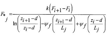.................(13)

where F is the variable (u, T or q) and i is the height of measurements adjacent; and ψ_m, ψ_h and ψ_v are, respectively, the stability correction functions for momentum, temperature and specific humidity, of Paulson (1970) and Dyer (1974); based on the measurement of two levels, k is the von Karman constant (= 0.40), so that:

.................(14)

..................................(15)

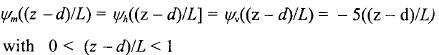..........................(16)

The Monin–Obukhov length, L, was obtained using the gradient Richardson number of each layer, j (Kaimal and Finnigan, 1994; Dyer and Hicks, 1970):

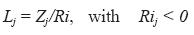.................................................(17)

........................(18)

The residual of the energy balance (g(Z_j/h)) can be plotted against any parameter we choose (for example, the canopy or soil temperature) in order to ascertain the relationship between them. Daamen et al. (1999) used a similar procedure to study the influence of a shelter and Cellier and Brunet (1992) to locate the inertial sublayer.

The residual in energy balance g(Z_j/h) plotted against the temperature difference (T_h) is between the bare soil surface temperature midway between the rows (T_is) and the soil surface temperature under the plants (T_sc); the rationale being that the horizontal temperature is linked to convective activity within the canopy and thus it explains the lack of balance in the lowest layer of the internal boundary layer. The relation between the residual, g(Z_j/h) and T_h is presented in Figure 9, for two relative heights (Z_j/h = 1 and 1.5). The g(Z_j/h) obtained from equation (10) is not dependent of T_h but from Figure 9 we can see that it is connected with T_h. The value of the residual was close to zero when Th was close to zero, which happened during the afternoon (after 15:30 h). The largest residuals were computed when the temperature (T_h) difference exceeded 20 °C.

The relative magnitude of w_* to that of the friction velocity allows us to recognize the cases for which the sensible heat generated at the bare soil could reach the layers above the canopy. We excluded these cases, and the vertical variation in g(Z_j/h) for the remaining ones is presented in figures 10 and 11, for unstable and stable cases, respectively.

Mahrt (2000) defined the thermal blending height for unstable conditions as directly proportional to the surface heat flux and inversely proportional to the wind speed. Results presented in Table III indicate that during unstable conditions the average residuals are not statistically different from zero for Z_j/h=1.9 to 2.4. These results are consistent with those of Kaimal and Finnigan (1994), and Cellier and Brunet (1992), who reported that when unstable conditions prevailed the roughness sub–layer extended until about twice the canopy height.

During the period when stable conditions prevailed (afternoon) the average residuals are not statistically different from zero for Z_j/h=1.5 to 2.4. This lowering of the lower boundary may be due to the combination of high wind speeds and a decrease in convective activity. The latter is a result of the fact that the canopy casts a shadow on the bare soil surface between the rows, thus decreasing the horizontal differences in soil surface temperatures. The inhomogeneity of the canopy seems to decrease due to both effects. Cellier and Brunet (1992) deduced the correction factor y of the universal functions (derivate above smooth surfaces), where is applied in the roughness sublayer. The for the sensible and latent heat flux result both equal to , where Z^* is the roughness layer depth. Taking the inter–row spacing δ=0.36 m, we obtain Z^*/δ=3.2 and 2.5 for unstable and advection conditions.

In Figure 12 the vertical variation of the residuals is presented for the cases for which the conditions that could lead to free convection inside of the canopy were observed [(u_* – w_*)<–0.02 and C₀>16]. These values were day 256 between 12:00 h and 14:30 h, and day 257 at 10:00 and 10:30 h. At the lowest levels, the residuals were significantly different from zero (Fig. 12), negative values for the lowest level, and positive ones for the intermediate one. The uppermost layer showed an extremely large variability. Extremely unstable conditions (Ri<–0.05) prevailed during these periods at the lowest level above the crop. The strong unstable condition can help the thermals emanating from the surface to reach the heights of measurements. This could be an explanation for the lack of balance in the energy equation. These results suggest that for this particular canopy and environmental condition (high soil surface temperature and relatively low wind speed) fluxes of sensible and latent heat could not be computed using the conventional flux–gradient relationships.

The residuals of the two uppermost layers are significantly less than zero for both, stable and unstable conditions. This could be due to insufficient fetch during the early morning (unstable conditions, Fig. 10) but not in the afternoon during which the wind blew from the NW. During this period, the lack of balance can only be ascribed to advection. The influence of advection can be estimated by the horizontal heat transport and is compared with the (vertical) sensible heat flux (H_a3). The horizontal heat transport approximates to ˜ T_a3•u₃ where the subindex 3 is the highest level of air temperature and wind speed observed. It is compared in Figure 13 with H_a3, observing that when H_a3 is negative a linear relation with horizontal transport exists, and there is a poor relation when H_a3 is positive. For that reason, when H_a3<0, the sensible heat flux has a component of horizontal heat transport, being an advection situation.

Finally, using the Bowen ratio (β₀) it is possible to compute the sensible (H_b) and latent (E_b) heat fluxes as:

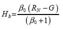..................................................................(19)

......................................................................(20)

where and is the psychrometric constant. Blad and Rosenberg (1974) concluded that when –2.5<Ri<0.025, the relation between the turbulent transfer coefficients for heat and water vapour, k_h/k_v, is close to 1 and the error in the Bowen estimation is <10%. The Richardson numbers (Ri) for the layer Z/h=1.9 do not exceed 0.02.

The equations (19) and (20) have to be applied at the level where the balance equation closes. H_b and E_b were evaluated at Z_j/h=1.9 of day 255 (Fig. 14) where the balance equation closes and there is no free convection. After 14:00 h the sensible heat flux (H_b) is negative and the latent heat flux (E_b) is higher than the available energy (R_N – G). The β₀ was negative after 14:00 h, while β₀ was lower than –1 between 17:30 and 18:00 h. The former is a characteristic value of advection condition with E_b>R_N – G, while the latter situation is the transition to a nocturnal stable condition (sunset) (Pérez et al., 1999). The interval around β₀=–1 can produce unreliable values of latent and sensible heat fluxes. Figuerola and Berliner (2005) present an extensive discussion about the error of the Bowen ratio.

 

3.4. Systematic error

The systematic error of the sensible heat flux and the friction velocity are analyzed. The expressions of the systematic error in relation with the displacement height length (d), the wind speed, and the temperature are deduced in the appendixes. Applying error analysis to H_a (Eq. 12), its error (δH_a) is given by:

.....................(21)

where ΔT = T_i+1 – T_i and Δu = u _i+1 – u _i, correspond to H_a of the layer j.

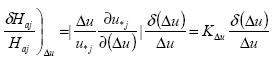
The relative error of H_a may be related to the relative error in the selected input parameter (p) (Figuerola and Mazzeo, 1997):

.......................................................................(22)

and the coefficient K_p is obtained by applying propagation of error analysis. Our case is δp equal to δd, δ(Δu) and δ(ΔT) results:

.......................................................................(23)

.................................................................(24)

................................................................(25)

where the coefficients K_d, K_Δu and K_ΔT were deduced in te annexes. δd=0.05 m and δ(Δu)=2δu and δ(ΔT)=2δT with δu=0.11 ms^–1 and δT=0.02°C.

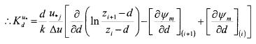
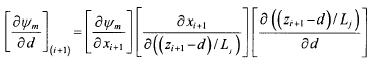
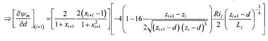
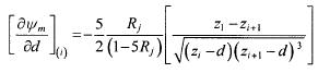
The relative error of H_a to the displacement height d (Eq. 23) can be rewritten as (A1):

.....................................(26)

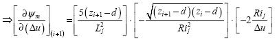
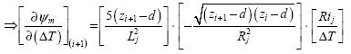
K_d^u* is defined by equation (A3) with (A4) and (A5) to the unstable and stable cases, respectively. While as K_d^T* is defined by equation (B2) with (B3) and (B4) to the unstable and stable cases, respectively. Figure (15) shows the K_d^u* and K_d^T* values with Z/h, the maximum occurs closer to canopy top, Z/h=1. According to our data δd/d=0.13, the mayor relative errord are 16 and 23% in unstable and stable conditions at Z/h=1. The error decrese, being 10% at Z/h=1.9. These results affirm that the error in H_a, due to the error in d, is bigger near the canopy top and it decreases with height.

The relative error of the friction velocity (u_*) respect to d results:

.....................................(27)

The K_d^u* is the same equation (A3) (Fig. 15), near the canopy top in the extreme case results K_d^u*˜ 1, and δd/d=0.13, then δu_* /u_* due to d is not so big. It is about 0.13 in unstable cases.

The K_Δu coefficient of the equation (24) is defined by the equation (C2) with (C3) and (C4) for the unstable and stable cases, respectively. In addition, the K_ΔT coefficient of the equation (25) is defined by the equation (D2) with (D3) and (D4). K_Δu and K_ΔT shown in Figure 16 as, function of the stability parameter Z/L. The highest unstable condition results in K_Δu˜ 0.5 and K_ΔT˜ 1.5. In neutral stability (– 0.01 < Z/L < 0.01), K_Δu and K_ΔT are about 1. Neutral stability is more probable to occur near of the canopy top, and the unstable conditions increase with height although high instability can occur in free convection near the canopy top. If strong stable conditions prevail, K_Δu increases and K_ΔT decreases.

The largest Δu and ΔT value's are near the canopy, as result the relative errors 2δu/Δu and 2δT/ΔT are small, increasing with height. According to equations (24) and (25) δH_a/H_a are big when ΔT or Δu are so small as two times the instrumental error. ΔT is small (< 2δ T) at noon when change of sign occurs, or Δu is small when free convection takes place.

In the afternoon, stability conditions between 0 < Z/L < 0.01 prevail on the lower layer (Z/h < 2.4) and ΔT and Δu are big and δH_a/H_a< 1. The same way we can say that the error of latent heat flux depends of error 2δq/Δq, being significant after 17:00 h.

The application of flux–profile relationships have lower error at Z/h < 2.4 than at Z/h > 2.4 when Δz is 0.5 m. Inversely, the error due to d is big at the lower high, but in our case the former error was more important that this latter.

The same as equation (27), but with relation to Δu, results in:

..........................................................(28)

According to equation (28), δu_*/u_* is < 1 (Fig. 17) when Z/h < 2.4, except in free convection cases (see Z/h = 1.5). We calculate δu_*˜ 0.7 ms^–1 if Z/h < 2.4 and δT_*˜ 0.6°C are the greatest values observed.

 

4. Conclusions

The study was carried out in an irrigated field planted with tomato, which was surrounded by large tracts of dry, bare soil. The crop was planted in rows and irrigated by trickle irrigation. The effects of these features on the surface boundary layer above the crop were researched on a number of selected days.

The gradients in temperature and water vapor pressure were obtained at various heights above the canopy using a Bowen ratio machine. This area is influenced by the sea breeze. The maximum temperature difference between the sea and desert land is about midday (maximum radiation), which generates a strong wind component. The hot air arrives on a cooler crop and the temperature gradient of the highest layer changes of sign at midday, and later in the lowest layer. The layer Z/h=3 receives the entrance of dry air from the desert area and the evapotranspiration induces a strong cooling in the bottom.

The fluxes of sensible and latent heat for several heights were computed applying the aerodynamic method. The residual in the energy balance equation was used as a criterion to determine the internal equilibrium layer.

Mixed convection conditions occurred from morning to midday (u_* > w_*) inside the canopy and weak unstable conditions above it. The closure of balance energy equation is between Z/h ˜1.9 to 2.4. The enclosure for Z/h < 1.9 was associated with inhomogeneous temperature in the soil of the canopy. The temperature differences between soil under the plants and bare soil between rows can arrive to 20 °C. During the late morning in short periods, the bare soil between the rows reached extremely high temperatures and low wind speeds occurred above the canopy (u_*< 0.16 ms^–1), and thus free convection inside was the dominant transport regime (w_*>u_*) during some hours. Z/h = 1.5 and 2.4 were different from zero and an extremely large variability was evident for the Z/h = 3.2 layer, no finding the equilibrium layer. Strongly advective conditions prevailed during the afternoon, manifested as an increase in the stability of the uppermost measured layer, and propagated slowly downwards. The closure of balance energy equation for the stable conditions above the canopy was between Z/h ˜ 1.5 and 2.4. The lowering of the equilibrium boundary for stable conditions was ascribed to the high wind speed and the fact that horizontal gradients in the soil surface temperature were small due to canopy shading, prevailing mixed and forced convection inside the canopy. In these cases, the inhomogeneous canopy did not have influence at the height 1.5 h. The residuals were significantly different from zero for the uppermost layers (Z/h = 2.7 and 3.2) during these periods.

Our findings suggest that the location of the equilibrium layer above fields surrounded by dry bare areas and in which row crops are trickle irrigated, vary in response to wind speed and the temperature of the soil between the rows of the crop, and that for some time intervals the estimation of fluxes may not be possible.

 

Acknowledgements

P. Figuerola received during her visit at the Jacob Blaustein Institute of the Ben Gurion University of the Negev a fellowship from the FOMEC (University of Buenos Aires, Argentina) and from the CONICET (National Council for Science and Technology, Argentina). This study was as well partly supported by GLOWA–JR.

 

Appendix A

..............................................................(A1)

....................................................................(A2)

whit F = u(wind speed) equation 13, and Δu = u_i+1– u_i

.........................(A3)

where

The unstable case: and , where

results:

and with

.....(A4)

The stable case: , with

and

.........................(A5)

 

Appendix B

................................................................................(B1)

being:

...................(B2)

The unstable case: where and

...........(B3)

and

The stable case: and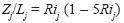

...........................(B4)

 

Appendix C

.........................................(C1)

with F = u (wind speed) equation 13, and Δu = u_i+1 – u_i

...................(C2)

The unstable case:

.....(C3)

The same to

The stable case:

...................................(C4)

 

Appendix D

.....................................................(D1)

To F = T (temperature) equation 13, and ΔT = T_i+1 – T_i, result:

............(D2)

The unstable case:

...........(D3)

The satable case: and

..........................(D4)

 

References

Bradley E. F., 1968. A micrometeorological study of velocity profiles and surface drag in the region modified by a change in surface roughness. Q. J. R. Meteorol. Soc. 94, 361–379.        [ Links ]

Blad B. L., and N. J. Rosenberg, 1974. Lysimetric calibrations of the Bowen ratio–energy balance method for evapotranspiration estimation in the central Great Plains. J. Appl. Meteorol. 13, 227–236.        [ Links ]

Brutsaert W. H., 1982. Evaporation into the atmosphere. Reidel, Dordrecht, Netherlands, 299 p.        [ Links ]

Businger J. A., J. C. Wyngaard, Y. Izumi, and E. F. Bradley, 1971. Flux–profile relationships in the atmospheric surface layer. J. Atmos. Sci. 28, 181–189.        [ Links ]

Cellier P. and Y. Brunet, 1992: Flux–gradient relationships above tall plant canopies. Agric. Forest Meteorol. 58, 93–117.        [ Links ]

Daamen C. C., W. A. Dugas, P. T. Prendergast, M. J. Judd, K. G. McNaughton, 1999. Energy flux measurement in a sheltered lemon orchard. Agric. Forest Meteorol. 93, 171–183.        [ Links ]

Dyer A. J. and B.B. Hicks, 1970. Flux–gradient relationships in the constant flux layer. Q. J. R. Meteorol. Soc. 96, 715–721.        [ Links ]

Dyer A. J., 1974. A review of flux–profile relationships. Boundary–Layer Meteorol. 7, 363–372.        [ Links ]

Dyer A. J., and T. V. Crawford, 1965. Observations of climate at a leading edge. Q. J. R. Meteorol. Soc. 91, 345–348.        [ Links ]

Elliott W. P., 1958. The growth of the atmospheric internal boundary layer. Trans. Amer. Geophys. Union, 39, 1048–1054.        [ Links ]

Figuerola P. I. and N. A. Mazzeo, 1997. Analytical model for predicting nocturnal and short after sunrise temperature of surface with near calm and cloudless sky. Agric. Forest Meteorol. 85, 229–237.        [ Links ]

Figuerola P. I. and P. R. Berliner, 2005. Evapotranspiration under advective conditions. Int. J. Biometeorol. 49, 6, 403–416.        [ Links ]

Ford E. D., 1976. The Canopy of a scots pine forest: description of a surface of complex roughness. Agric. Forest Meteorol. 17, 9–32.        [ Links ]

Garrat J. R., 1979. Comments on the paper "Analysis of flux–profile relationships above tall vegetation–an alternative view" by B. B. Hicks, G. D. Hess and M. L. Weseley. Q. J. R. Meteorol. Soc. 105, 1079–1082.        [ Links ]

Hebbar S. S., B. K. Ramachandrappa, H. V. Nanjappa and M. Prabhakar, 2004. Europ. J. Agronomy, 21, 117–127.        [ Links ]

Hicks B. B., G. D. Hess and M.L. Wesely, 1979. Analysis of flux–profile relationships above tall vegetation–an alternative view. Q. J. R.Meteorol. Soc. 105, 1074–1077.        [ Links ]

Jacobs A. F. G. and N. Verhoef, 1997. Soil evaporation from sparse natural vegetation estimated from Sherwood numbers. J. Hydrology, 188–189, 443–452.        [ Links ]

Jacobs A. F. G., J. H. Van Boxel and R. M. El–Kilani, 1994. Nighttime free convection characteristics within a plant canopy. Boundary–Layer Meteorol. 71, 375–391.        [ Links ]

Jegede O. O. and T. Foken, 1999. A study of the internal boundary layer due to a roughness change in neutral conditions observed during the LINEX field campaigns. Theor. Appl. Climatol. 62, 31–41.        [ Links ]

Kaimal J. C. and J. J. Finnigan, 1994. Atmospheric boundary layer flows, their structure and measurement. Oxford. Univ. Press, 289 p.        [ Links ]

Kroon L. J. M. and N. J. Bink, 1996. Conditional statistics of vertical heat fluxes in local advection conditions. Boundary Layer Meteorol. 80, 50–78.        [ Links ]

Kustas W. J., B. J. Bhaskar, K. E. Kunkel and LL. W. Gay, 1989. Estimate of the aerodynamic roughness parameters over an incomplete canopy cover of cotton. Agric. Forest Meteorol. 46, 91–105.        [ Links ]

Lee X. Q. Yu, S. Xiaomin, L. Jiandong, M. Qingwen, L. Yunfen and X. Zhang, 2004. Micrometeorolo–gical fluxes under the influence of regional and local advection: a revisit. Agric. Forest Meteorol. 122, 111–124.        [ Links ]

Mahrt L., 2000. Surface heterogeneity and vertical structure of the boundary layer. Boundary–Layer Meteorol. 96. 33–62.        [ Links ]

Mayocchi C. L. and K. L. Bristow, 1995. Soil surface heat flux: some general questions and comments on measurements. Agric. Forest Meteorol. 975, 43–50.        [ Links ]

Monteith J. L, M. H. Unsworth, 1990. Principles of environmental physics, 2nd ed. Edward Arnold, London, 291 p.        [ Links ]

Mulhearn P. J., 1977. Relations between surface fluxes and mean profiles of velocity temperature, and concentration, downwind of a change in surface roughness. Q. J. R. Meteorol. Soc. 103, 785–802.        [ Links ]

Panofsky H. A., 1965. Re–analysis of Swinbank's Kerang observations: Flux of heat and momentum in the planetary boundary layer. Rept., Dept. of Meteorology, Penn. State Univ. 224 p.        [ Links ]

Paulson C. A., 1970. The mathematical representation of wind speed and temperature profiles in the unstable atmospheric surface layer. J. Appl. Meteorol. 9. 857–861.        [ Links ]

Pérez P. J., F. Caste llvi, M. Ibáñez and J. Rosell, 1999. Assessment of reliability of Bowen method for partitioning fluxes. Agric. Forest Meteorol. 97, 141–150.        [ Links ]

Perrier E. R., J. M. Robertson, R. J. Millington and D. B. Peters, 1972. Spatial and temporal variation of wind above and within a soybean canopy. Agric. Forest Meteorol. 10, 421–442.        [ Links ]

Prueger J. H., L. E. Hipps and D. I. Cooper, 1996. Evaporation and the development of the local boundary layer over an irrigated surface in an arid region. Agric. Forest Meteorol. 78, 223–237.        [ Links ]

Rana G. and N. Katerji, 2000. Measurement and estimation of actual evapotranspiration in the field under Mediterranean climate: a review. Europ. J. Agronomy. 13, 125–153.        [ Links ]

Raupach M. R., 1979. Anomalies in flux–gradient relationships over forest. Boundary–Layer Meteorol. 16. 467–486.        [ Links ]

Raupach M. R., 1991. Rough–wall turbulent boundary layers. Appl. Mech. Rev. 44, 1–25.        [ Links ]

Robinson S. M., 1962. Computing wind profile parameters. J. Atmos. Sci. 19. 189–190.        [ Links ]

Schween J. H., M. Zelger, B. Wichura, T. Foken and R. Dlugi, 1997. Profiles and fluxes of micrometeorological parameters above and within the Mediterranean forest at Castelporziano. Atm. Environ. 31, 185–198.        [ Links ]

Shuttleworth W. J. and J. S. Wallace, 1985. Evaporation from sparse crops–an energy combination theory. Q. J. R. Meteorol. Soc. 111, 839–855.        [ Links ]

Stull R. B., 1988. An Introduction to boundary–layer meteorology. Kluwer, Dordrecht, 666 p.        [ Links ]

Thom A. S., 1975. Momentum, mass and heat exchange of plant communities vegetation and the atmosphere. In: Vegetation and the atmosphere (J. L. Montheit, Ed.) Academic Press, London, 57–110.        [ Links ]

Zangvil A., Z. Offer, I. A. Osnat Mirón, A. Sasson and D. Klepach, 1991. Meteorological analysis of the shivta region in the Negev, Desert Meteorology Papers, Series B No 1, Ben–Gurion University of the Negev. The Jacob Blaustein Inst. 202 p.        [ Links ]

Zelger M., J. Schween, J. Reuder, T. Gori, K. Simmerl and R. Dlugi, 1997. Turbulent transport, characteristic length and time scales above and within the Bema forest site at Castelporziano. Atm. Environment. 31, 217–227.        [ Links ]