Probabilistic description of rains and ENSO phenomenon
in a coffee farm area in Veracruz, México

 

J. L. BRAVO, C. GAY, C. CONDE and F. ESTRADA
Centro de Ciencias de la Atmósfera, Universidad Nacional Autónoma de México
Circuito exterior, Ciudad Universitaria, México D. F., México 04510 México
Corresponding author: J. L. Bravo; e–mail: jlbravo@atmosfera.unam.mx

 

Received September 2, 2005; accepted November 16, 2005

 

RESUMEN

Se analizan 37 años de datos climáticos con el objetivo de describir el comportamiento de la precipitación y su relación con la temperatura en una región productora de café en el estado de Veracruz, en particular en los municipios de Coscomatepec y Huatusco. Se analizan las tendencias de los promedios anuales de la precipitación. Los promedios mensuales de precipitación se relacionan con la temperatura promedio mensual para emplear a la temperatura como un parámetro útil para predecir las lluvias intensas. Se ajustan distribuciones gama a la precipitación total mensual que permiten aproximar el cálculo de probabilidades para intervalos dados de precipitación. Así mismo se ajustaron distribuciones Gumbel a los valores extremos diarios para periodos mensuales y a valores extremos mensuales para periodos anuales. Se analiza la relación de la precipitación con el fenómeno de El Niño Oscilación del Sur (ENOS) encontrándose influencia causada por la disminución de la sequía interestival (canícula) en presencia de años de Niño.

 

ABSTRACT

We have analyzed 37 years of climate data to describe the behavior of the precipitation and its relation with temperature in coffee farm areas in the central part of the state of Veracruz, particularly in the municipalities of Coscomatepec and Huatusco. We analyze the tendencies of the annual averages of the precipitation. Monthly averages of the precipitation are related with monthly averages of the temperature as useful parameters to predict intense rains. Gamma distributions were adjusted to total monthly precipitation to approximate the probability of given intervals. Gumbel distributions were adjusted to daily extreme values for monthly intervals and to monthly extremes for annual intervals. The relation of the precipitation and the El Niño/Southern Oscillation (ENSO) phenomenon is analyzed. The influence of ENSO over the precipitation was found to be significant and translated as a reduction of the midsummer drought.

Keywords: Veracruz, coffee farms, precipitation trends, probabilistic forecast, ENSO influence, extreme precipitation values.

 

1. Introduction

The utilization of forecast of climatic variables in planning activities in different sectors is becoming more frequent as our understanding of some oceanic–atmospheric phenomena has improved in recent years as is the case of the El Niño or ENSO (El Niño/Southern Oscillation). Major research centers are capable of producing reasonable forecasts of the El Niño phenomenon with six months anticipation that are available to the public through their internet websites (National Center for Environmental Prediction, Climate Prediction Center, International Research Institute for Climate Prediction). This information can be very useful as the effects of this event on regional or local climate can be estimated in order to anticipate their influence on different activities.

The impacts of El Niño in México, in general terms, are well known (Magaña, 1999; Escobar et al., 2001). During El Niño years winters carry more precipitation than normal particularly in the north of the country where the cold season may also be intense. In contrast, during summer, the precipitation is lesser and the temperature is higher than during normal years in most of the country, accompanied by severe droughts that affect water availability and agricultural activities. These effects are less masked in a strong El Niño event.

Although the impacts of El Niño in México have been well described in general terms, its effects at regional or local level are mostly unknown. Useful forecasts need this information to make them applicable for productive activities such as agriculture.

The relationship between the temperature and the precipitation and how El Niño affects these variables is explored in this work for a particular region in México where coffee is grown. This paper describes the behavior of precipitation and its relation with the temperature measured at 8:00 h, local time, in a coffee production region in the state of Veracruz, in particular the municipalities of Coscomatepec and Huatusco. The relationship between the precipitation and ENSO phenomenon is also described.

An important factor in cultivating coffee is precipitation and a significant mater is its trend. A systematic one, comes as a result of the global climate change, and could affect the conditions for coffee development and its quality. The optimal precipitation for the Arabica variety, that is mainly cultivated in the area, is between 1500 and 2500 mm per year with dry periods that favor the blossom. Adequate annual mean temperatures are between 18 and 24 °C (Nolasco, 1985).

The 1992 Coffee Census (Consejo Mexicano del Café, 1996) reveals that in Veracruz 153,000 hectares are devoted to coffee production, involving 67,000 producers from 82 municipalities and generating around 300,000 permanent jobs and 30 million daily wages each year (Gay et al., 2004).

The area of study is in the state of Veracruz, that is located in the central coast of the Gulf of México. It limits to the North with the state of Tamaulipas, to the West with the states of San Luis Potosí, Hidalgo and Puebla, to the south with the states of Oaxaca and Chiapas, and to the east with Tabasco state and the Gulf of México. Veracruz has mountainous areas with a steep slope towards the Gulf of México as could be seen in level curves of Figure 1. The study area is located between 18° 49' and 19° 48' N, and 96° 30' and 97° 13' W. The stations in that area are located at altitudes from 311 to 1842 masl. The period of observation goes from 1961 to 1998.

 

2. The data

The analyzed data were taken from the ERIC II (Quintas and Ramos, 2000) database. The temperature measurements for Huatusco and Coscomatepec turned out to be not reliable as it is shown later. It was then necessary to use the temperature measured at 8:00 h and the daily precipitation from eight auxiliary neighboring stations. Their geographical positions are listed in Table I and shown in Figure 1.

 

3. Results

3.1 Characteristics of precipitation in Huatusco and Coscomatepec

Annual means of the total monthly precipitation at Huatusco and Coscomatepec are shown in Figure 2.

Trends of precipitation at Huatusco and Coscomatepec are weak; the first is decreasing while the second increases. The trends are not significant at 5% confidence level for both stations (–0.08 ± 0.31 and 0.16 ± 0.34 mm/year respectively).

Figure 3 shows monthly averages of total precipitation for the whole period. The relative reduction during August, known as the "canícula" or midsummer drought, described earlier by Mosiño and García (1966), and by Magaña et al. (1999), is clearly illustrated. Table II shows the monthly means (mm/month), standard deviation and coefficient of variation of precipitation in both locations. These values are consistent with those obtained by Tejeda et al. (1989) for January, April, July and October.

Coefficient of variation shows homogeneous values for months June, July, August and September that correspond to the period of regular rains and shows no homogeneous values for the rest of the year. This could be due because during those months the rains are stable and during the rest of the year the rains are scarce and irregular.

3.1.1 Characteristics of the statistical distribution of precipitation in Huatusco and Coscomatepec

Gamma distribution (Hogg and Craig, 1978; Wilks, 1995) is represented by the following formula:

...........................................(1)

b is a scale parameter, c is a shape parameter and is the gamma function. This theoretical distribution was adjusted to monthly precipitation values for the 37 years of data for Huatusco and Coscomatepec stations. Adjustments were satisfactory according to the chi square criterion (Conover, 1980). There was homogeneity in the shape and scale values of the adjusted parameters for the months of June, July, August and September and also during the months of November, December, January, February, March and April, which correspond to the rainy and dry seasons respectively. The months of May and October are considered of transition between precipitation regimes and are considered separately. Table III shows the adjusted parameters.

This probability distribution function allows to calculate the probabilities of occurrence of certain ranges of the precipitation. Empirical probability distribution functions for the stations are presented in Appendix.

Gumbel distributions (Reiss and Thomas, 2001; Buishand, 1989; Wilks, 1995) were fitted for extreme daily values (the greatest precipitation daily value) for each month of the two stations. Gumbel distributions are frequently used to model extreme values and have the following density probability distribution:

....................................(2)

Where a is a location parameter an d is a scale parameter.

Table IV shows location and scale parameters for Huatusco and Coscomatepec. In Gumbel distributions the location parameter is equal to the mode of the distribution expressed in daily millimeters of precipitation.

As it was mentioned before the adjusted parameters are homogeneous for the rainy season. A new Gumbel distribution was adjusted for the extreme values of the rainy months and for each station. This procedure allow us having more data for the adjustment considering the months of the rainy season as a replication of a rainy month. Figure 4 shows the fitted Gumbel curves to the extreme values during rainy and dry seasons.

Location and scale parameters for Huatusco and Coscomatepec are shown in Table V for the entire sets of rainy and dry seasons. The fitting was acceptable using the chi squared criteria.

Notice in Figure 4 the small secondary maximum to the right of the histograms that represents the highest precipitation during the 37 years study period. These values could represent a second mode of the extreme precipitation distribution caused by a different physical phenomenon like hurricanes that landed in points near the area of study. There were five daily precipitation values between 160 and 180 mm/day in Huatusco and five daily values between 120 and 160 mm/day. This information could be used for risk assessments and for prevention of damages caused by intense precipitation during daily periods.

Gumbel distributions were adjusted to each year extreme values, adjustment parameters and graphs are shown in Figure 5 and Table VI. Adjustments are not rejected at 0.05 confidence using chi square test.

These fitted functions permit the calculation of probabilities of extreme dangerous daily precipitations during a month or a year. Tables VII and VIII are numerical calculations for the probabilities for precipitation grater than X extreme values expressed in mm.

Also in Figure 5 there are small secondary maximum to the right of the histograms that represent highest precipitation during the 37 years study period. As mentioned earlier these values could represent a second mode that is clearer in Huatusco.

The extreme precipitation values are dangerous, especially above 130 mm; when this value is reached, the civic protection authorities issue a "declaration of emergency". These were the cases of torrential rains from 1–3, May, 2004 and from October 31, to November 13, 2003 (reported in the Diario Oficial de la Federación, 2003, 2004).

 

3.2 The relationship between precipitation and temperature

The relationship between precipitation and temperature could be used for predicting precipitation using the conditional function of probability distribution. Figure 6 shows monthly–cumulated precipitation versus the monthly means of temperature. This figure shows that there is a threshold of temperature under which precipitation values bellow 100 mm/month does not occur. Since the temperature is not reliable for Huatusco and Coscomatepec, the data of eight auxiliary stations were used for comparative purposes. Examples of this behavior are shown in figures 7 and 8 (Actopan and Jalcomulco). Some stations like Atzalán, shown in Figure 8, do not show this threshold.

Figures 6 and 7 show that precipitation greather than 100 mm/month in Actopan and Jalcomulco, occurs only for temperatures above 20 °C. In the case of Atzalán this sharp contrast is not clear and precipitation above 100 mm/month can occur at farther low temperatures (8 to 9 °C). In fact, precipitation above 100 mm/month in respect to the incoming winds of the gulf coast, as is shown in Figure 1, could be the reason for the differences in precipitation vs. temperature behavior among stations.

In Atzalán the precipitation is larger in comparison with Actopan and Jalcomulco, this may be because Atzalán is very high and exposed to the North winds that cause precipitation above 100 mm/month.

The value of the threshold of temperature is not constant for all stations that show it. The temperature threshold is lower as the altitude of the station increases (Fig. 9), as could be expected due to the reduction of temperature with the altitude.

This behavior of temperature and precipitation suggests that values of temperature above certain thresholds could be used in the probabilistic forecast for strong precipitation and compared with a probabilistic forecast made with the rainy season (June, July, August and September). We selected those months with monthly mean temperature higher than the threshold for locations where this behavior is present. Using those months we constructed the empirical functions of probability distribution (EFPD) (Conover, 1980) for each location. The season of the year can also be used to predict precipitation, and then EFPD were also calculated for the months of the rainy season. These functions are shown in Appendix. The combination of both criteria can be used to calculate the EFPD for the months that have temperatures greater than the threshold during the rainy season. We also calculated the EFPD for the total rainy season. The combination of temperature and season of the year are better than any single criterion because is more restrictive than the individual ones.

The use of EFPD allows calculating the probability of occurrence of any interval of precipitation using the mentioned criteria of temperature and/or season of the year. Using data of Appendix it is possible to calculate the probability of a given precipitation during a month or during the entire rainy season. The calculated values are in accordance with the probabilities obtained by Tejeda et al. (1989) in the area of study.

 

3.3 Precipitation and ENSO phenomenon relationship

Most of the meteorological parameters show seasonal variation. Then, when a correlation coefficient between two monthly means of meteorological parameters is obtained they will show a certain level of association, even though there is not a real relationship between them. The same effect occurs when both variables show trends. To eliminate the seasonal variation it is possible to average a seasonal period. As we mentioned earlier, Huatusco has a non–significant decreasing precipitation trend in yearly mean values and the Multivariate ENSO Index (MEI) (Wolter, 1987; Wolter and Timlin, 1998) shows also a significant increasing trend. Being this so, the correlation coefficient between them should be negative, however, the calculated correlation coefficient is 0.42, that is significant. Eliminating trends in both data series the correlation coefficient is 0.47. We calculated the correlation coefficient between the MEI series including its trend, and the de–trended precipitation series obtaining 0.46. Those values suggest a relation between precipitation and MEI in Huatusco. Years with larger MEI values have more precipitation.

Yearly means in Coscomatepec do not have significant precipitation trends. The correlation coefficient of yearly means of MEI with yearly means of precipitation was 0.36 and with de–trended MEI was 0.35. This suggests also that precipitation increases when MEI increases.

Huatusco and Coscomatepec were the only two stations with significant correlation coefficient for the MEI. Table IX shows the correlation matrix of the MEI and precipitation yearly means for auxiliary stations.

Another way to eliminate the seasonal variation is to classify observations in months, and calculate correlation coefficients for each month. Note that these 12 series could have trends that could be eliminated assuming linear trends. Table X shows the significant values of the de–trended correlation coefficients for Huatusco and Coscomatepec using numbers 1 or –1 for positive or negative values respectively, and 0 when their value is not significant. Cells are empty when both correlation coefficients are not significant.

Huatusco and Coscomatepec precipitation in July is positively correlated with MEI conditions from March to September. That is, it rains more with ENSO conditions in July. On the other hand precipitation decreases in October with MEI values during March and April. In the case of Coscomatepec there is also a positive relation of precipitation with MEI values in August and September and a negative relation of December precipitation with MEI values for January, February and March.

 

3.4 Estimation of precipitation using the Multivariate ENSO Index

As we mentioned earlier, MEI yearly mean has a marked increasing trend. If we suppose a linear trend the following regression can be calculated

.............................(3)

This fitting is only valid for the studied period and could be extrapolated to short intervals if conditions do not change. It is possible to calculate the residuals of this regression and use them as a predictor for estimating total yearly precipitation in Huatusco and in Coscomatepec. The results are shown in equations (4) and (5).

Huatusco:

........(4)

Coscomatepec:

........(5)

Standard errors of estimation are 201.3 and 273.2 respectively.

To make an estimation of precipitation, we first estimate the deviation of the MEI observed value from a forecasted MEI value and then calculate an estimated precipitation using equations (4) or (5) for Huatusco or Coscomatepec.

Using annual mean MEI values for the 1998–2000 period, we estimated total precipitation and confidence intervals for Huatusco (Draper and Smith, 1981). These values were compared with the observed ones. The comparison is made in Table XI. Observed values for 1998–2000 are inside the calculated 95% confidence interval. There are no reliable values for precipitation in Coscomatepec for the 1998–2000 period.

 

3.5 Relation between the midsummer drought in Huatusco and Coscomatepec with ENSO phenomena

We found the months of midsummer drought by means of plotting monthly values of precipitation for years from 1961 to 1997 for both stations. During some years, the phenomenon was not present. For years when the phenomenon is present we evaluate their intensity drawing a line between the two ridges of the midsummer drought precipitation depression and we obtain the difference between the interpolated values using the drawn line and the observed values during the period of the phenomenon (Mosiño and García 1966; Magaña et al. 1999). The sum of these differences is approximately proportional to the area represented by the midsummer drought and we call it the midsummer drought intensity.

The correlation coefficients between the intra–seasonal drought intensity and the corresponding MEI value for the middle month of the intra–seasonal drought period was significant and negative for Huatusco, values are shown in Table XII. This means that for bigger values of MEI low values of the intra–seasonal drought intensity are to be expected. This result supports the finding mentioned earlier that bigger values of MEI seems to be related with an increase in July precipitation.

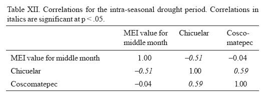
The correlation coefficient between the two stations intra–seasonal drought intensity shows the relation between the rain of the stations. The coefficient between intensity of intra–seasonal drought phenomenon and MEI shows that for larger values of MEI there must be low values of the intensity of the intra–seasonal drought. This implies a larger total precipitation for that year.

 

3.6 End of dry season and ENSO phenomenon

We combined the graphs of Huatusco and Coscomatepec and found the last two weeks of the dry season for each year. Figure 10 shows the relation between MEI values during the last observed dry month vs. the number of the last two weeks of the observed dry season for each year.

During the considered period there were only five strong ENSO phenomena (1983, 1987, 1992, 1993 and 1997, marked with large dots in the graph). During these years the dry season ends during the ninth "two week" period of the year or later. In other words: with strong ENSO phenomenon the rainy season in the study area did not start early.

 

4. Conclusions

• Precipitation for Huatusco and Coscomatepec show a very weak trend. The former is decreasing and the latter increasing (–0.08 ± 0.31 and 0.16 ± 0.34 mm/year respectively) and therefore no significative changes in yearly totals of precipitation are expected in next years.

• Gamma functions properly describe the density probability functions for monthly values of precipitation when they are fitted to rainy season (June to September), to dry season (November to April) and for a transition stage (October and May).

• Gumbel functions properly describe the probability density functions for the extreme values of daily precipitation during a month for the rainy season. The probability of surpassing 130 mm during a day (that is a condition for a declaratory of emergency action) is of considerable value (0.259) during a year and lower (0.053) during a month of the rainy season.

• There could be a small second mode in the distributions of extreme precipitation and it may be caused by hurricanes that enter near to the area of study.

• Temperatures measured at 8:00 h that surpass a threshold are useful parameters to make a probabilistic forecast for precipitation. The EFPD compared with the EFPD for precipitation during the rainy season (June to September) is another criterion to make a probabilistic forecast.

• The MEI values for months from May to September and the precipitation during July show a marked positive correlation.

• The MEI values could be useful to estimate total yearly precipitation in Huatusco and Coscomatepec by means of linear relations. Observed values are inside the calculated 95% confidence intervals for the period 1998–2000.

• The rainy season does not start early in years with strong ENSO phenomenon. However this is not the only cause of that behavior.

 

Acknowledgments

We thank to Víctor Zarraluqui for his useful suggestions with data and maps, to María de Lourdes Godínez for the elaboration of maps and to Beatriz Elena Palma for the useful data supplied.

 

Appendix

 

References

Buishand T. A., 1989. Statistics of extremes in climatology. Stat. Neerl. 43, 1–30.        [ Links ]

Conover W. J., 1980. Practical nonparametric statistics. Second Edition, Wiley, New York, 462 p.        [ Links ]

Consejo Mexicano del Café –Secretaría de Agricultura, Ganadería y Desarrollo Rural, 1996. México Cafetalero. Estadísticas Básicas. México.        [ Links ]

Diario Oficial de la Federación, 17–junio–2004.         [ Links ]

Diario Oficial de la Federación, 17–diciembre–2003.        [ Links ]

Draper N. R. and H. Smith, 1981. Applied regression analysis. Second Edition, Wiley, New York, Chapter 1, 709 p.        [ Links ]

Escobar E., M. Bonilla, A. Badán, M. Caballero and A. Winckell, 2001. Los efectos del fenómeno El Niño en México: 1997–1998. Consejo Nacional de Ciencia y Tecnología, México, 246 p.        [ Links ]

Gay C., F. Estrada, C. Conde, H. Eakin and L. Villers, 2004. Potential impacts of climate change on agriculture: A case of study of coffee production in Veracruz, México. Climatic Change. Submitted.        [ Links ]

Reiss R.–D and M. Thomas, 2001. Statistical analysis of extreme values. Second Edition, Birkhäuser Verlang, Boston, 440 p.        [ Links ]

Hogg R. V. and A. T. Craig, 1978. Introduction to mathematical statistics. Collier Macmillan, London, 103–108.        [ Links ]

Magaña V. O., 1999. Los impactos de El Niño en México. Dirección General de Protección Civil, Secretaria de Gobernación, México, 229 p.        [ Links ]

Magaña V., J. A. Amador and S. Medina, 1999. The midsummer drought over México and Central America. J. Climate, 12, 1577–1588.        [ Links ]

Mosiño A. P. and E. García, 1966. Evaluación de la sequía intraestival en la República Mexicana. Proc. Conf. Reg. Latinoamericana Unión Geogr. Int. 3, 500–516.         [ Links ]

Nolasco M., 1985. Café y sociedad en México. Centro de Ecodesarrollo, 1985, 94–95 p.        [ Links ]

Quintas I. and D. Ramos, 2000. Extractor rápido de información climatológica (ERIC). Instituto Mexicano de Tecnología del Agua, Subcoordinación de Desarrollo Institucional, Progreso, Morelos, México.        [ Links ]

Soto M. and E. García, 1989. Atlas climático de estado de Veracruz. Instituto de Ecología, Xalapa, Veracruz, México. 125 p.        [ Links ]

Tejeda A., F. Acevedo and E. Jáuregui, 1989. Atlas climático del Estado de Veracruz, Universidad Veracruzana, México, 150 p.        [ Links ]

Wilks S. D., 1995. Statistical methods in the atmospheric sciences. Academic Press, New York. 467 p.        [ Links ]

Wolter K., 1987. The Southern oscillation in surface circulation and climate over the tropical Atlantic, Eastern Pacific, and Indian Oceans as captured by cluster analysis. J. Climate Appl. Meteor. 26, 540–558.        [ Links ]

Wolter K., and M. S. Timlin, 1998, Measuring the strength of ENSO–how does 1997/98 rank? Weather 53, 315–324.        [ Links ]