On the annual cycle of the sea surface temperature and the mixed
layer depth in the Gulf of México.

 

V. M. MENDOZA, E. E. VILLANUEVA and J. ADEM
Centro de Ciencias de la Atmósfera, UNAM, Circuito Exterior, C. U., 04510, México, D. F., México
Corresponding author: V. M. Mendoza; e–mail: victor@atmosfera.unam.mx

 

Received March 1, 2004; accepted February 22, 2005

 

RESUMEN

Usando un modelo integrado en la capa de mezcla hemos obtenido una simulación del ciclo anual de la temperatura de la superficie del mar (SST), de la profundidad de la capa de mezcla (MLD) en el Golfo de México, así como del ciclo anual de la velocidad de penetración vertical turbulenta a través de la termoclina en la región más profunda del Golfo de México. El modelo se basa en las ecuaciones de conservación de energía térmica y mecánica, ésta última derivada de la teoría de Kraus–Turner, ambas ecuaciones están acopladas e integradas verticalmente en la capa de mezcla. Las ecuaciones del modelo se resuelven en una malla regular de 25 km en el Golfo de México, la región noroeste del Mar Caribe y la costa este de Florida. La velocidad de la corriente oceánica superficial y las variables atmosféricas son prescritas en el modelo usando valores observados. Mostramos la importancia que tiene el bombeo de Ekman en la velocidad de penetración turbulenta. Encontramos que la surgencia tiene un papel importante en incrementar la penetración turbulenta produciendo un enfriamiento del agua superficial y una disminución en la profundidad de la capa de mezcla en la Bahía de Campeche. En el resto del Golfo el hundimiento tiende a reducir la penetración turbulenta y a incrementar la temperatura de la superficie y la profundidad de la capa de mezcla. Una comparación del ciclo anual de la SST y de la MLD calculados con el modelo muestran concordancia con las correspondientes observaciones reportadas por Robinson (1973). En la región profunda del Golfo de México, los datos de concentración de pigmentos fotosintéticos, obtenidos de análisis ambientales, muestran en enero, abril, mayo junio y septiembre correlación significativa con el ciclo anual de la velocidad de penetración vertical turbulenta calculada.

 

ABSTRACT

Using an integrated mixed layer model we carry out a simulation of the annual cycle of the sea surface temperature (SST) and of the mixed layer depth (MLD) in the Gulf of México. We also compute the annual cycle of the entrainment velocity in the deepest region of the Gulf of México. The model is based on the thermal energy equation and on an equation of mechanical and thermal energy balance based on the Kraus–Turner theory; both equations are coupled and are vertically integrated in the mixed layer. The model equations are solved in a uniform grid of 25 km in the Gulf of México, the northwestern region of the Caribbean Sea and the eastern coast of Florida. The surface ocean current velocity and the atmospheric variables are prescribed in the model using observed values. We show the importance of the Ekman pumping in the entrainment velocity. We found that the upwelling plays an important role in increasing the entrainment velocity, producing an important reduction in the SST and diminishing the depth of the mixed layer in the Campeche Bay. In the rest of the Gulf of México the downwelling tends to reduce the entrainment velocity, increasing the SST and the MLD. Comparison of the computed annual cycle of the SST and the MLD with the corresponding observations reported by Robinson (1973), shows a good agreement. In the deepest region of the Gulf of México, the photosynthetic pigment concentration data obtained from the Mexican Pacific CD–ROM of environmental analysis shows significative correlation with the computed annual cycle of the computed entrainment velocity only in January, April, May, June and September.

Keywords: Sea surface temperature; mixed layer depth; Gulf of México.

 

1.  Introduction

We have used a model that is based in the thermal energy equation applied to the surface layer of the Gulf of México to simulate the annual cycle of sea surface temperature (SST) (Adem et al., 1991), the ocean–atmosphere heat fluxes (Adem et al., 1993), as well as to predict the SST anomalies and their month–to–month changes in the Gulf of México (Adem et al., 1994), obtaining some degree of skill in the simulations and predictions.

The incorporation in the model of the Kraus and Turner (1967) theory and of the Alexander Woo–Kim hypothesis (Niiler and Kraus, 1977; Kim, 1976) to compute the cooling in the mixed layer by entrainment through the thermocline improves the skill of the simulations of the SST anomalies, mainly for the summer and the fall seasons (Mendoza et al., 1997). Other authors as Zavala et al. (2002) have studied the average and seasonal variation of the heat fluxes and the SST in the Gulf of México, considering the relative importance of the heat advection and the entrainment.

This work is a contribution to modeling of the ocean upper layer using an integrated mixed layer model based in the thermal energy equation instead of one based in the hydrodynamic equations, such as was proposed by Blumberg and Mellor (1983), Price et al. (1978), Price (1983), Price and Weller (1986), and Bender and Ginis (2000). The advantage of this model is that has a less computational cost and provides a method to show the importance of the entrainment mechanism and the Ekman pumping on the annual cycle of the SST and the mixed layer depth (MLD).

 

2.  Mixed–layer model

The ocean mixed layer is the top layer which is well mixed by wind, so that we can assume that it has a vertically uniform temperature. The mixed layer thickness (h) is defining the depth at which a sharp gradient of temperature indicates the start of the thermocline. The bottom of the mixed layer allows a mass vertical flux across it, defined as entrainment (if upwards).

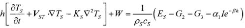
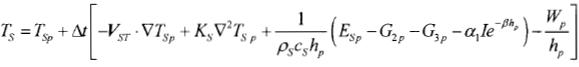
The equation for the prediction of the month–to–month changes of SST in the Gulf of México is the conservation of thermal energy equation given by:

........(1)

where T_S is the SST, V_ST the horizontal velocity of the ocean currents in the mixed layer, the two dimensional gradient operator, K_S the constant horizontal exchange coefficient, W the rate of cooling in the mixed layer due to turbulent vertical penetration of colder water from the thermocline, E_S the rate at which the energy is added by radiation, G₂ the rate at which the sensible heat is given off to the atmosphere by turbulent transport, G₃ the rate at which the heat is lost by evaporation, β is the solar extinction coefficient, and is the solar radiation absorbed by the layer. When the absorption is complete , this case has been used in a previous paper by Mendoza et al. (1997). The water density, and the specific heat, c_S, are considered constant and equal to 1.035 kg m^–3 and 4186.0 Jkg^–1K^–1 respectively.

The last term, in the right side of equation (1), is the penetrative radiation in the layer and has been neglected in a previous paper by Mendoza et al. (1997).

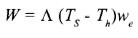
The entrainment term W, in equation (1) can be expressed by:

............................................................(2)

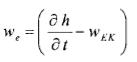
Where w_e is the entrainment velocity which in agreement with Alexander (1992) is associated with the mixed layer deepening modified by Ekman pumping velocity w_EK, and is given by:

............................................................(3)

Where is the Heaviside function given by:

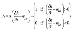............................(4)

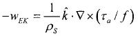
In equation (2), T_h is the sea temperature below the mixed layer, which is assumed constant and equal to 288.15 K(15 °C); and w_EK is Ekman pumping velocity given by:

...............................................(5)

Where is the downward vertical unit vector; , the surface wind stress vector; and f=2Ωsinφ, the Coriolis parameter; Ω, the angular velocity of the Earth and φ, the latitude.

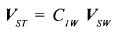
For the horizontal ocean currents in the mixed layer we shall assume that:

.................................................................(6)

Where C_IW is an empirical coefficient and V_SW is the horizontal velocity of the seasonal surface ocean current, which is prescribed in the model using observed values. We use C_IW=0.235, assuming that the currents in the Gulf of México have a vertical profile in the whole frictional layer similar to the pure drift current (Adem, 1970).

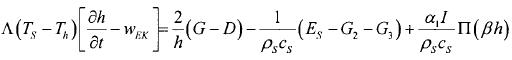
The other equation of the model represents a balance between mechanical energy and thermal energy, where the entrainment of colder water is determined according to Kraus and Turner (1967) by:

.....(7)

Where G is the turbulent kinetic energy input from the wind, D is the dissipation within the layer, and is the solar penetration function. On the left–side of equation (7), the first term represent the rate of working needed to lift and mix the denser entrained water; on the right–hand side the first term represent the balance between the wind generation and dissipation of turbulent kinetic energy, and the second and third terms represent the rate of potential energy change produced by the net heating and the penetration of solar radiation in the mixed layer.

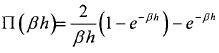
The solar penetration function in equation (7) is given by:

............................................(8)

Alexander and Woo Kim (1976) found realistic results of mixed layer depth in the North Pacific Ocean using β=0.1m^–1, therefore we assuming this value for the Gulf of México, because this value represents very well the typical ocean–water in depths greater than 50 m according to Jerlov (1951,1968).

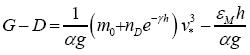
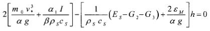
The difference between the rate of generation and dissipation of turbulent kinetic energy is given in accordance with Alexander and Woo Kim by:

.......................................(9)

Where =2.1 x 10^–4K^–1 is the thermal expansion coefficient of sea water; g=9.8 ms^–2, the acceleration of gravity; m₀=1.25, an empirical parameter; n_D= 1.25 and =0.05 m^–1, parameters of dissipation; v_* the frictional velocity related to the surface wind stress by Alexander and Woo Kim obtained optimal results of the mixed layer depth in the summer season, using a parameter of background dissipation ε_M=2.0x10^–8m²s^–3, which exists even in the absence of wind stress; we found the best results with ε_M=2.0x10^–8m²s^–3 for spring, ε_M=3.2x10^–8m²s^–3 for summer and ε_M=0 for fall and winter.

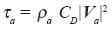
For the surface wind stress, we use the bulk formula (Isemer and Hasse, 1987):

.................................................................(10)

Where and are the surface air density and the surface wind speed, respectively; and C_D, the atmospheric drag coefficient.

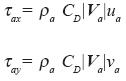
The components west–east and south–north of the wind stress vector are, respectively, given by:

..............................................................(11)

Where u_a and v_a are the components west–east and south–north of the surface wind vector, respectively.

 

2.1 The heating function

The rate at which the energy is added by radiation at the sea surfac (ES) is computed as Budyko (1974):

......(12)

Where =0.96 is the emissivity of the sea surface: , the Stefan–Boltzmann constant; T_a , the surface air temperature; U, the surface air relative humidity; e_ST_α, the saturation vapor pressure at the surface air temperature in hPa; ε, the fractional amount of cloudiness; and c=0.65, a cloud cover coefficient.

For the solar radiation absorbed by the ocean layer , we use the Barliand–Budyko equation:

..............................(13)

Where (Q + q)₀ is the total solar radiation received by the surface with clear sky; , the albedo of the sea surface; and a and b are the coefficients taken from Budyko (1974). The coefficient a is a function of the latitude and the coefficient b is a constant equal to 0.38. For the Gulf of México we use a=0.35, which corresponds to 25 °N of latitude.

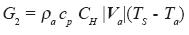
The heating functions G₂ and G₃ are given by the following equations (Mendoza et al, 1997):

..................................................(14)

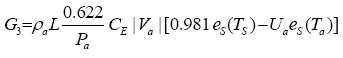...................(15)

Where c_p=1.004 Jkg^–1K^–1 is the specific heat of air at constant pressure; L=2.44 x10⁶Jkg^–1, the latent heat of vaporization which is considered constant; P_a, the sea level pressure; C_H and C_E, the vertical turbulent transport coefficients of the sensible and latent heat, respectively. The coefficients C_D, C_H and C_E are determined according with Huang (1978) by:

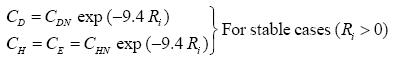.............................(16a)

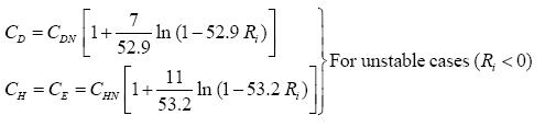.........(16b)

Where C_DN =2.5x10^–3 and CHN = 1.2x10^–3 are the drag coefficient for momentum and sensible heat for the neutral case, respectively, and R₁ is the bulk Richardson number given by:

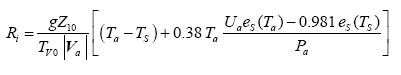............................(17)

Where Z₁₀=10 m and T_V0=298 K are the reference height and the reference temperature in the Richardson number, which is also a function of the surface wind speed and the virtual air–sea temperature difference, where the correction of the virtual temperature is applied to T_a.

In equations (15) and (17) the saturation vapor pressure is computed using the follow equation (Adem, 1967):

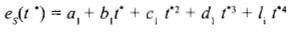.............................(18)

where e_S(t^*) is in millibars and t^* is the temperature in Celsius degree; a₁= 6.115, b₁= 0.42915, c₁= 0.014206, d₁=3.046x10^–4 and l₁= 3.2x10^–6.

 

2.2 The integration method

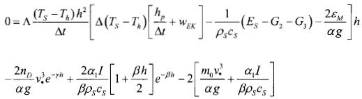
Equations (1) and (7) are applied to time–averages of one month in a uniform grid on the sea surface of the Gulf of México, the north–western of the Caribbean Sea and the Atlantic Ocean region contiguous to Florida (Fig. 1). For the time integration we apply for equation (1) the explicit Euler method and for equation (7) a backward implicit time finite difference scheme, therefore for equation (1) we obtain:

............(19)

And for equation (7):

........................(20)

Where we use (8) and (9) in (7) to obtain equation (20) and where Δt is the time–step which is taken of 2 hours; the sub–index p indicate that T_S and h take values of the previous time step.

In a previous work (Mendoza et al, 1997) we used equation (20) with =0, and assuming that 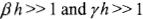, we computed diagnostically the MLD and its effect in the monthly prediction of the SST anomalies. In this case equation (20) is reduced to:

........................(21)

Therefore:

....................................................(22)

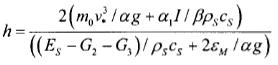
For summer and fall, equation (22) yields results in agreement with the observations of Robinson (1973); however, for winter and spring we obtain discrepancies between the MLD values computed from equation (22) and those observed. These results suggest that the MLD must be computed, mainly for winter and spring, of the complete equation (20).

In this work to compute h from equation (20), we use the successive approximation method of Newton (Carnahan et al, 1969).

To simulate the annual cycle of T_S and h, we start the computations in January by assuming that h=60 m, T_S=298.15 K (25°C) and that the cooling by entrainment is equal to zero (W_P = 0) in equation (19).

With T_S computed in the first time–step from equation (19), we compute h from equation (20) taking = 1, which is verified if the first condition in (4) is satisfied. In this way we obtained T_S and h for the first time–step; however, if the second condition in (4) is satisfied, then we compute again h taken now =0 in equation (20).

For the second time–step, we take as initial condition T_S and h from the first time–step. The process is continued until completing one month, with 360 time–steps of 2 hours.

The temperature T_S and the depth h computed in the last time–step is now used as initial condition to compute the temperature and the depth for February, and so on.

This iteration process is continued for several annual cycles until the temperature and the depth computed for each month between two consecutive years have a difference smaller than 0.01 °C and 0.01 m, respectively. These conditions are achieved after a run of 5 years.

For the spatial derivatives in equation (19), we use centered differences with a regular grid of 25 Km where the horizontal transport of heat by ocean currents and by turbulent eddies are taken as zero at the points in the closed boundaries (coasts). At the points in the open boundaries (in the Caribbean Sea and Atlantic ocean regions contiguous to Florida), we assume that the horizontal transport of heat by turbulent eddies is zero. For the horizontal transport of heat by ocean currents in the open boundaries, we compute the term using climatic observed values of the surface ocean currents and the sea surface temperatures.

 

2.3 Input–data

For the horizontal velocity vector of the surface ocean currents V_SW (Fig. 2), we use the compiled data from the Oceanographic Atlas of the Mexican Marine Office (1985).

For the components u_a and v_a of the surface wind; as well as for the surface air temperature, T_a and the surface relative humidity, U_a, we use monthly values from NOAA–CIRES, Climate Diagnostic Center of Boulder Colorado (CDC) (Web site at http://www.cdc.noaa.gov/). The wind speed computed with the components u_a and v_a results greater that the wind speed reported by NOAA–CIRES CDC; this inconsistency has been eliminated using for seasonal values derived from the revised maps of scalar wind speed taken from the Bunker Climate Atlas of the North Atlantic Ocean, (Isemer and Hasse, 1987), which does not include the components of the surface wind.

Seasonal values of the fractional amount of cloudiness, e, and the albedo of the sea surface, , were obtained from data files of the Adem's thermodynamic climate model (Adem, 1965).

 

3. Results and discussion

3.1 SST, MLD and the entrainment velocity fields

We computed the annual cycle of the SST and the MLD from equations (19) and (20), respectively, and compared the results with the corresponding observed average data reported by Robinson (1973). As examples we show the cases of January and July corresponding to winter and summer, respectively. Figure 3 shows the SST, in Celsius degrees, computed for January (Part A) and the corresponding observed values (Part B). Figure 4 is as Figure 3 but for July.

The comparison of part A with part B, for the case of January and July, shows that the model has some skill to simulate the SST.

In January, it is clearly shown the effect that on the SST has the water flow through the Yucatán Channel, associated with the Loop Current (Fig. 3, Part B). This effect on the SST has been, in part, simulated by the model due to the prescribed observed currents. In the central part of the Gulf of México the model simulates temperatures very close to the observations. However in the Texas–Louisiana shelf it is observed a more pronounced northward cooling than the one computed by the model. Temperatures approximately uniform of 29°C are observed in July (Fig. 4, Part B), decreasing one degree toward the west coast of the Gulf, and toward the Yucatán and Florida shelves. The model also simulates approximately uniform temperatures of 29°C in the center of the Gulf, with a decrease towards the northeast, however the temperatures simulated by the model over the Campeche Bay of up to 27 °C (Fig. 4, Part A) are not observed in the Part B of Figure 4. These low temperatures, over the Campeche Bay, simulated by the model are produced by a relatively strong upwelling (Fig. 8, Part B), that produces an important entrainment of cold water from the thermocline (Fig. 9, Part B).

Figure 5 shows the MLD, in meters, computed for January (Part A) and the corresponding observed values (Part B). Figure 6 is as Figure 5 but for July. For January, the model yields minimal values of MLD in the Campeche Bay and in the North of Florida and yields maximal values in the Texas Shelf between Corpus Christi and Mississippi Delta. Also it yields maximal values to the south of Florida and around the island of Cuba, which has certain agreement with the observations (Fig. 5, Part B). For July the thermocline is considerably shallower than in January. In this case the result of the model is between about 15 and 30m in the Gulf of México and of the order of 45m in the northwest portion of the Caribbean Sea, which is also in agreement with the observations.

In accordance with equation (22), to a first approximation, h is proportional to v_*³/(E_S–G₂–G₃), therefore in July, maximal values of h (Fig. 6, part A) tend to coincide with maximal values of (Fig. 7A) and minimal values of the heating (E_S–G₂–G₃) in the central part of the Gulf (Fig. 7B).

Figure 9 shows the entrainment velocity (10^–6 ms^–1) computed by the model for January (Part A) and July (Part B). In January, values higher than 3x10^–6 ms^–1 in the entrainment velocity are located over the Texas–Louisiana Shelf and towards the north of the Campeche Bay (Fig. 9A), whereas in July (Fig. 9B) they are only located in a reduced area towards the north of the Campeche Bay.

In order to determine the degree of cooling of the mixed layer, as well as its changes in depth, we have made an experiment in which the Ekman pumping velocity is neglected in Equation (20). Figure 10, shows the difference between the entrainment velocity, computed taking into account the Ekman pumping velocity, and the one computed neglecting it. In all the Campeche Bay, but mainly towards the north part, the upwelling plays an important role in increasing the entrainment (positive values in Figure 10), and producing a maximal reduction in the temperature of 1.5°C for January (Fig. 11 A) and of 3.0°C for July (Fig. 11B). In the rest of the Gulf of México the downwelling (positive values in Fig. 8) tends to reduce the entrainment velocity and to increase the temperature up to 1.0°C in January and 2.0°C in July, as is shown in Figure 11.

Figure 12 shows that the upwelling tends to diminish the depth of the mixed layer in the Campeche Bay and, the downwelling tends to increase the depth of the mixed layer in the rest of the Gulf of México. The most important changes in the depth of the mixed layer due to either upwelling or downwelling occur in January (Fig. 12A).

 

3.2 The annual cycle of the SST, the MLD and the entrainment velocity

Next we will show the annual cycle of the SST, MLD and entrainment velocity using spatial averages month to month. Figures 13 and 14 show the computed and the observed annual cycle of the SST and of the MLD, respectively, in the basin of the Gulf of México, delimited by the open boundaries shown by the line B1 in the Yucatán Channel and the line B2 in the Florida Strait (Fig. 1). The computed annual cycle of SST (Fig. 13) shows, in agreement with the observations, a variation of 8 °C between February and August, with a minimum value in February and a maximum in August. The MLD shows a variation of 57 m with a minimum value of 19 m in July and a maximum of about 78 m in February (Fig. 14).

The photosynthetic pigment concentration, obtained from the Mexican Pacific CD–ROM of environmental analysis, is used for comparison with the computed entrainment velocity. Since we did not take into account the photosynthetic pigment concentration due to the rivers and lagoons, this comparison is carried out in the deepest closed region of the Gulf of México delimited by the polygon shown in Figure 1.

Photosynthetic pigment concentration in the deepest region of the Gulf of México (Fig. 15), exhibits maximum values in winter (December, January and February) and minimum values in summer (June, July and August), which is in agreement with the annual cycle of the entrainment velocity. The entrainment velocity shows a maximum in May, which is slightly hinted in the photosynthetic pigment concentration.

Figures 16 and 17 show the annual cycle of the SST and the MLD in the deepest region of the Gulf of México. These curves exhibit a monthly variability similar to the one of the whole basin of the Gulf of México (Figs. 13 and 14).

The agreement between the computed and the observed annual cycle shown from figures 13 to 17 (13, 14, 15, 16, 17)does not imply that the spatial distribution of the computed and the observed variables have a similar agreement. Therefore, we have evaluated the similitude between the computed and observed spatial distribution of the SST, and the MLD, using the index of agreement (Appendix A), and the normalized correlation coefficient between the entrainment velocity and the observed photosynthetic pigment concentration. The index of agreement is not a measure of correlation in the formal sense but rather a measure of the degree to which a model's predictions are error free, at the same time is a standardized measure to estimate the error, regardless of units. It varies between 0.0 and 1.0 where a computed value of 1.0 indicates perfect agreement between the observed and predicted observations, and 0.0 connotes one of a variety of complete disagreements.

Figure 18 shows the index of agreement between the SST computed by the model and the SST observed in the basin of the Gulf of México (solid line) and in the deepest region of the Gulf of México (discontinues line), for all months of the year. These curves indicate that in the whole basin of the Gulf of México, the index of agreement is more significant mainly from October to May (0.8–0.9) than from June to September (0.4–0.5). A similar configuration is observed for the deepest region but with significant values of the index of agreement only from January to May. The low agreement in the deepest region is due probability to the horizontal transport of thermal energy by the anticyclonic eddies shaded of the Loop Current, which is not included in the model.

Figure 19 is similar to Figure 18, except that for the MLD. This figure indicates that in the whole basin the index of agreement is significant (0.5–0.8) from February to July while that in the rest of the year, the index is not significant ( < 0.4). In the deepest region of the Gulf of México there are significative values (0.5–0.6) only in June and July.

Figure 20 shows the normalized correlation coefficient between the entrainment velocity and the photosynthetic pigment concentration in the deepest region of the Gulf of México delimited by the thick line shown in Figure 1, the comparison month to month between the spatial distribution of entrainment velocity and photosynthetic pigment concentration, shows a significant positive correlation only in January, April, May, June and September. The significant positive correlation may be due in part to the entrainment of colder water, rich in nutrients, from the thermocline which is raising the concentration of photosynthetic pigments.

 

4. Concluding remarks

Alexander and Woo–Kim applied the Kraus and Turner theory to compute the MLD in the North Pacific Ocean for summer in the region where the entrainment could be considered as zero, and therefore the MLD was determined from a diagnostic equation, in which the SST was prescribed using observed values. In this work we compute the MLD from equation (7), which includes the entrainment (=1), and which is coupled with the thermodynamic equation, from which the SST is computed. Therefore our model is able to simulate with certain skill the basic characteristics of the SST and the MLD throughout the whole year. Here we have shown only the results for January (winter) and July (summer).

We have shown the importance of the Ekman pumping in the entrainment velocity; we found that the upwelling plays an important role in increasing the entrainment velocity, producing in the Campeche Bay, an important cooling in the SST and diminishing the depth of the mixed layer. In the rest of the Gulf of México the downwelling tends to reduce the entrainment velocity, increasing the SST and the MLD.

The computed annual cycle of the SST and the MLD in the whole basin of the Gulf of México shows some agreement with the observations.

We found a significant positive correlation between the computed entrainment velocity and the observed photosynthetic pigment concentration in January, April, May, June and September which may be due in part to the entrainment of colder water, rich in nutrients from the thermocline, which is raising the concentration of photosynthetic pigments.

Good results have been obtained recently (unpublished paper), applying this model to the study of the effect of cold air–outbreaks, tropical storms and hurricanes on the SST and the MLD in the Gulf of México.

 

Acknowledgements

We are indebted to Berta Oda Noda, Alejandro Aguilar Sierra and Rodolfo Meza for the computational technical support.

 

Appendix A

The index of agreement d (Willmott and Wicks, 1980) is expressed as:

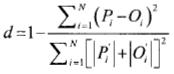
Where O_i is the observed variable, P_i is the predicted variable. The index of agreement d, specifies the degree to which the observed deviations about (observed means) correspond, both in magnitude and sign, to the predicted deviations about 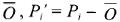and .It is assumed that the portions of the magnitudes P_i and O_i that are equivalent to are not in error since is considered to be error free.

 

References

Adem, J., 1965. Experiments aiming at monthly and seasonal numerical weather prediction. Mon. Wea. Rev. 93, 495–503.        [ Links ]

Adem, J., 1967. Parameterization of atmospheric humidity using cloudiness and temperature. Mon. Wea. Rev. 95, 83–88.        [ Links ]

Adem, J., 1970. On the prediction of mean monthly ocean temperature. Tellus 22, 410–430.        [ Links ]

Adem, J., Mendoza, V. M., Villanueva Urrutia, E. E, Monreal–Gómez, M. A., 1991. On the simulation of the sea surface temperature in the GulfofMéxico using a thermodynamic model. Atmósfera. 4, 87–99.        [ Links ]

Adem, J., Villanueva, E. E., Mendoza, V. M., 1993. A new method for estimating the seasonal cycle of the heat balance at the ocean surface, with application to the Gulf of México. Geofís. Int. 32, 21–34.        [ Links ]

Adem, J., Villanueva, E. E., Mendoza, V. M., 1994. Preliminary experiments in the prediction of sea surface temperature anomalies in the Gulf of México. Geofís. Int. 33, 511–521.        [ Links ]

Alexander, M. A., 1992. Midlatitude atmosphere–ocean interaction during El Niño. Part I: The North Pacific Ocean. J. Climate, 944–958.        [ Links ]

Alexander, R. C., Jeong–Woo Kim, 1976. Diagnostic model study of mixed–layer depths in the summer North Pacific. J. Phys. Ocean. 6, 293–298.        [ Links ]

Bender, M.A. and Ginis, I., 2000. Real–case simulation of hurricane–ocean interaction using a high–resolution coupled model: effects on hurricane intensity. Mon. Wea. Rev. 128, 917–946.        [ Links ]

Blumberg, A. F. and Mellor G. L., 1983. Diagnostic and prognostic numerical circulation studies of the South Atlantic Bight. J. Phys. Res. 88, C8, 4579–4592.        [ Links ]

Budyko, M. I., 1974. Climate and Life. International Geophysics Series, 18, Academic Press, New York. 508 pp.        [ Links ]

Carnahan, B., Luther, H. A., Wilkes, J. O., 1969. Applied Numerical Methods. John Wiley & Sons, INC. 604 pp.        [ Links ]

Huang, J. C. K., 1978 Numerical simulation studies of oceanic anomalies in the North Pacific Basin, I. The ocean model and the long–term mean state. J. Phys. Oceanogr. 8, 755–778.        [ Links ]

Isemer, H. J., Hasse, L., 1987. The Bunker Climatic Atlas of the North Atlantic Ocean, Vol. 2. Air–Sea Interactions. Springer–Verlag, Berlin, 252 pp.        [ Links ]

Jerlov, N. G., 1951. Optical studies of ocean water. Rept. Swed. Deep–Sea Exped., 3, 1–59.        [ Links ]

Jerlov, N. G., 1968. Optical Oceanography. Elsevier, 199 pp.        [ Links ]

Kim, J. W., 1976. A generalized bulk model of the oceanic mixed layer. J. Phys. Ocean. 686–695.        [ Links ]

Kraus, E. B., Turner, J. S., 1967. A one–dimensional model of the seasonal thermocline, II. The general theory and its consequences. Tellus 19, 98–106.        [ Links ]

Mendoza, V. M., Villanueva, E. E., Adem, J., 1997. Numerical experiments on the prediction of the sea surface temperature anomalies in the Gulf of México. J. Mar. Sys. 13, 83–99.        [ Links ]

Niiler, P.P., Kraus, E. B., 1977. One–dimensional models of the upper ocean. Modelling and Prediction of the Upper Layers of the ocean. E. B. Kraus, Ed., Pergamon Press, 143–172.        [ Links ]

Price, J. F., Mooers, C. N. K., Van Leer, J. C., 1978. Observation and simulation of storm–induced mixed layer deepening. J. Phys. Ocean. 8, 582–599.        [ Links ]

Price, J. F., 1983. Internal wave wake of a moving storm. Part I: scales, energy budget and observations. J. Phys. Ocean. 13, 949–965.        [ Links ]

Price, J. F., Weller, R. A., 1986. Diurnal cycling: observations and models of the upper ocean response to diurnal heating, cooling and wind mixing. J. Geophys. Res. 91, C7, 8411–8427.        [ Links ]

Robinson, M. K., 1973. Atlas of monthly mean sea surface and subsurface temperature and depth of the top of the thermocline Gulf of México and Caribbean Sea. Scripps Inst. Ocean., Univ. California, San Diego, SIO Ref. 73–8.        [ Links ]

Willmott, C., Wicks, D. E., 1980. An empirical method for the spatial interpolation of monthly precipitation within California. Phys. Geogr. 1, 59–73.        [ Links ]

Zavala–Hidalgo J., Parés–Sierra, J., Ochoa, J., 2002. Seasonal variability of the temperature and heat fluxes in the Gulf of México. Atmósfera 15, 81–104.        [ Links ]