Stochastic analysis of time series of temperatures in the
south-west of the Iberian Peninsula

 

L. GARCÍA BARRÓN
Departamento de Física Aplicada II, Universidad de Sevilla, España
e-mail: leoncio@us.es

M. F. PITA
Departamento de Geografía Física y A.G. R., Universidad de Sevilla, España

 

RESUMEN

Se han elaborado los modelos autorregresivos integrados de media móvil (ARIMA) para las series mensuales de larga duración, de temperaturas máximas y mínimas, de los observatorios del suroeste español. Se han transformado las series originales para hacerlas estacionarias. Se han obtenido los órdenes (p, d, q) para cada serie mensual y, tras los procesos de validación por medio de las series de residuos, también se han obtenido los parámetros de las funciones estimadas de los modelos estocásticos mensuales. Como consecuencia, se han formulado predicciones sobre su evolución: las previsiones de los modelos ARIMA inducen a esperar que la temperatura mínima en la región objeto de estudio se encuentra en una fase de incremento térmico medio previsto del orden de 0.2 °C en el próximo decenio. Sin embargo, no está definida significativamente la evolución de las temperaturas máximas. Estas estimaciones se corresponden con las obtenidas previamente por los autores, en estudios anteriores, por otros métodos, pero con mucha mayor precisión en este caso.

 

ABSTRACT

Autoregressive Integrated Moving Average (ARIMA) models have been devised for long-term monthly series of maximum and minimum temperatures from south-western Spanish observatories. The original series were transformed into stationary ones, and the orders (p, d, q) for each monthly series were obtained. These were validated using series of residuals, and the parameters of the functions were estimated from the monthly stochastic models. The forecasts of change formulated from the ARIMA models suggest that the minimum temperatures in the study area are in a mean warming phase of the order of 0.2 °C over the next decade. The change in maximum temperatures is not significantly defined. These estimations correspond with those obtained by the authors in earlier studies using other methods, but the level of precision is much higher in this case.

Key words: Stochastic processes; time series; climate change; Iberian Peninsula.

 

1.  Introduction

The aim of stochastic analysis of time series by the formulation of ARIMA models is to separate the observed elements into two components: The first contains the organized part, including the trend, and the second the random residuals. The models constructed following such separation are used in an attempt to explain the time structure of each series and predict its change. The time series is considered a set of observables of the variables -maximum and minimum temperatures-measured at regular intervals. In this study, temperature measurements made during the period of observation are grouped to form monthly series.

Each of the series must be tested as fulfilling the statistical conditions required by the Box-Jenkins method for such models. We then proceed to identify and estimate the corresponding parameters, so that the estimated model not only fits the observations well, but also enables forecasts to be made.

The theoretical basis of the proposed models, including the definition of conditions of applicability, deduction of equations, and significance of the results, has been set out by various authors (Chatfield, 1992; Box and Jenkins, 1970; Kendall and Ord, 1990; Wei, 1990; Uriel, 1995; Peña, 1995; Ferrand, 1997). Others have used autoregressive moving average techniques in sociology and economics, and also, to a lesser degree, specifically in the study of meteorological variables (Garrido and García, 1994; Al-awadhi and Jolliffe, 1998; Martín et al., 1998; Zekai, 1998, Bravo, et al., 2001; Greiser et al., 2002; Solange and Pinto, 1996).

The following section indicates the observatories used in this study and the characteristics of stationarity required for the time series. Section 3 briefly describes the methodological basis of Autoregressive Integrated Moving Average (ARIMA) processes. Section 4 determines the order for each series, the corresponding functions generated by the model, and the respective residual series. Some of them have been represented graphically as an example. Section 5 estimates, from the results obtained for each monthly series, the forecast for the following decade.

 

2. Data

The observatories selected for the study are those from south-west Spain (western Andalucía and the south of Extremadura) having data series of the order of a century (Fig. 1). The records are from Sevilla-Tablada (37° 22'N, 6° 00' W), Córdoba (37° 53'N, 4° 47'W) Badajoz (38° 53' N, 6° 58' W), and Huelva (37° 15', 6° 57'W). The series of variables analyzed are the monthly maximum and monthly minimum temperatures from 1882 to 1999. (As the Huelva observatory ceased activity in 1983, no prediction has been made in section 5 due to the lack of data for the final period).

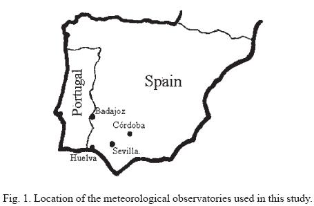
The data were previously subjected to a process of "gap-filling" and tested for uniformity (García-Barrón and Pita, 2001). We consider that these observatories characterize the south-western Iberian Peninsula climate, a region of interest owing to the Azores anticyclone direct action on it. Geo-graphically, the region is delimited by Lisbon and Gibraltar, continental points used by some authors to demonstrate the effects of the North Atlantic Oscillation (Hurrell, 1995; Pita López et al. 1999; Pozo-Vázquez et al., 2000).

It is a prerequisite that the time series be stationary before application of the Box-Jenkins method, so this must be verified and, if necessary, appropriate transformations made.

Accepting that the (X_t) series fluctuate around the mean value m that characterizes them, we can express the perturbations δ_t , as the differences between the observed values (x_t) and the µ value,

The process is considered stationary if, for any of the subseries ( X_ij) into which the complete time series is fragmented:

• the mean is constant -that is, the mathematical expectancy of the perturbation is zero.

• the variance is constant; in such case, the perturbation is denominated homocedastic.

•  the perturbations are independent of each other -that is, the correlation r_k between two observations, x_t and x_t+k , depends only on the number of lags separating them.

Furthermore, it is a requirement that the perturbations have a normal distribution, explicable by the central limit theorem, such that they cannot be imputed to specific causes but result from the effect of multiple random factors.

In the previous studies carried out (García-Barrón, 2000), we obtained the following results:

• Regarding the stability of the mean, most of the monthly series show a trend in the minimum temperatures (significant and with a slope coefficient between 1.7° and 3.3° per century, depending on month and observatory) and also in the maximum temperatures (although not constant in the sign of the slope, and with no statistical significance in some cases). It is therefore recommendable that all the series undergo first-order differencing to eliminate this trend (owing to the stability in variance a second derivation is not suggested).

• Regarding variance, the Levenne test shows that a great number of original series remain within the limits of stability, with a quasi-normal distribution. Nevertheless, logarithmic transformation generally improves variance, in particular in those series with homocedasticity not initially accepted.

Thus, to unify the procedure, the adaptation criterion for all the series will be a first-order linear derivation and logarithmic transformation. The Kolmogorov-Smirnov test confirms that the transformed monthly series fit the Gaussian distribution and can be accepted as meeting the requirement of normality.

Save the exceptions indicated below, the monthly series of maximum and minimum temperatures from the selected observatories fulfill the conditions required for stochastic analysis.

 

3. Stochastic processes

In the time domain, the series under study are considered as the specific result of a particular family of variables representing a statistical phenomenon that changes over time. Such family of variables is known as a stochastic process.

Any deductions from a single performance of the process require the imposition of restrictions: To be stationary in mean and variance and ergodic. Moreover, the sample must have an approximated normal distribution in order to satisfy the application rules in the autocorrelations of the later analysis. Stochastic processes can be represented as linear combinations of terms in which random variables take part, and, in particular, those formed by random pure processes (white noise), autoregressive processes, and moving average processes.

An autoregressive process of order p, denominated AR(p), is that in which a term of the series X_t be expressed as a linear combination of the preceding p terms plus one at random

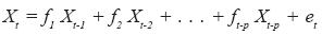
so that, using the linear operator of lag L X_t = X_t-1 gives

A moving average process of order q, denominated MA(q), is that in which a term of the series X_t can be expressed as a linear combination of the preceding random q terms

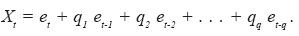
An ARMA (p, q) process is autoregressive, of moving average, from the combination of the former.

The reason for devising an ARIMA model is to find a function that, with a limited number of parameters, is a sufficiently close representation of how the observed series behaves.

The key mechamism for identifying a stochastic process is the calculation of the autocorrelation function (ACF) and partial autocorrelation function (PACF), that consider the values of the time series in relation with its lags, thereby revealing its inner structure. The values of the mean m and sampling covariances g_k establish the properties and relationships of the autocorrelation coefficients r_k for the corresponding processes AR(p), MA(q), and ARMA(p, q).

The autocorrelation coefficient, r_k, where k = 0, 1, . . . , indicates the lag interval between the terms of the series. The sequence of rk values constitutes the estimated autocorrelation function (or correlogram) calculated from the values of the series. When r_k is used as estimator of the stochastic processes, its distribution must be known in order to make inferences and to verify the significance of the different coefficients.

The partial autocorrelation coefficient (PACF) of order k is defined as the measurement of the linear relationship between k separate lags, independently of the intermediate values.

It is possible to demonstrate theoretically that in autoregressive AR(p) processes, a system of equations is obtained relating the first p coefficients of autocorrelation with the parameters Φ of the process (Yule-Waker equations). In autoregressive processes, the autocorrelation function decreases after a determined lag, geometrically or sinusoidally with possible alternation of sign, but without becoming zero. This makes it difficult to interpret the correlogram for establishing the order: It is necessary to use the function of partial autocorrelation coefficient. The Yule-Waker equations enable the coefficients Φ_i to be determined. The partial autocorrelation coefficients will be different from zero for lags not exceeding p, as by hypothesis the coefficients Φ₁, Φ₂, ..., Φ_p are non-zero.

In the moving average MA(q) processes, it is possible to obtain the relationship of the autoregression coefficients with the θ parameters of the model. Autocorrelation coefficients r_k are zero for lags above q, and the partial autocorrelation coefficients decrease exponentially and/or sinusoidally.

Thus, the behavior of the autocorrelation function of a MA process seems to be similar to that of the partial autocorrelation function of an AR process.

In the ARMA(p, q) processes, the identification of parameters is more complex because, generally, in the ACF or in the PACF the first values do not behave constantly and the following ones present damped oscillation, with no characteristic pattern. Although identifying mechanisms have been proposed, the most used system is that of comparison with the theoretical behavior of pre-established generative functions for values below p and q (Uriel, 1995).

The ARIMA (p, d, q) processes are ARMA (p, q) processes related to series that, not being initially stationary, have been subjected to an order-d differencing process. That is, an "integrated" process is denominated ARIMA (p, d, q) if, taking differences of order d, is transformed into an ARMA (p, q) -type stationary process.

Once the generative model is identified, the corresponding values of the parameters are calculated from the known correlation coefficients.

Fit is verified by adaptation of the model, using analysis of residuals -the difference between observed and obtained values. Ideal models are those of best fit with lowest number of parameters. There are two methods of verification: by autocorrelation of residuals, or by residual variance. Autocorrelation of residuals is based on their constituting white noise and random time distribution. Consequently, subjected to correlational analysis, all the coefficients of the correlogram of residuals must be within the confidence interval, being significantly zero. The alternative analysis of residual variance establishes the best order of the autoregressive model to avoid overfit. This addresses the significance of the extra variance explained by the introduction of a new parameter.

 

4. Application to the series of temperatures. Results

The presentation of the procedure and results follows the sequence of phases presented above.

4.1 Determination of order

We have stated that the order of the p autoregressive coefficients and of the q moving averages in each series is determined using the autocorrelation coefficients (ACF) and partial autocorrelation coefficients (PACF). Briefly, if the coefficients in the first q lags of the ACF are non-zero and the following ones are zero, and those of the PACF decrease exponentially or sinusoidally, we initially ascribe the series as MA(q). On the other hand, if the coefficients in the first p lags of the PACF are non-zero and the following ones are zero, and those of the ACF decrease exponentially or sinusoidally, we initially ascribe the series as AR(p). If the form of the ACF and PACF is a superimposition of those described, the model is denominated ARMA(p, q).

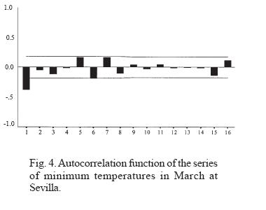
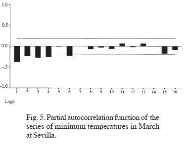
To avoid reiteration in the graphical display of the procedure and observations, whose results are implicit in the following tables, we will give later, as significant examples, only the monthly series of September and March of the minimum temperatures from the Sevilla observatory (Figures 2, 3, 4, 5).

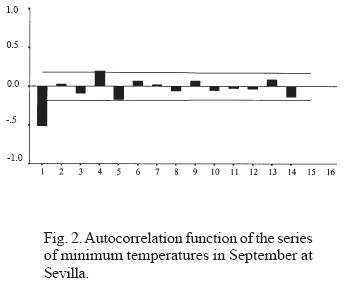
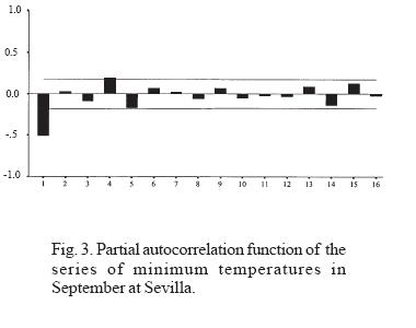
As the analysis is referred to monthly and annual series, which do not present stationarity, we determine the orders of the ARIMA(p, d, q) models. Because the series present a trend, they are subjected to first-order differencing so that, in such cases, d = 1.

The graphs (Figures 2-5: 2, 3, 4, 5) display the simple autocorrelation and partial autocorrelation functions of the minimum temperatures for the months of September and March at Sevilla. The first conclusion suggests both series belong to an MA(1) model, since only the first lag of the ACF is significantly different from zero (although one of the later retards is very close to the level of confidence). The shape of the first lags of the ACF is descending. However, calculation of the corresponding coefficients shows that the case of September leads to a state at the limit of invertibility (the theoretical condition for rejecting the model). Thus, we reformulate the model as AR(3), since the three autoregressive coefficients prove to be significant. Given that the series are subject to a trend, we introduce first-order differencing and conditionally accept models of type (3,1,0) for September and (0,1,1) for March. In both cases, logarithmic transformation is used to guarantee homocedasticity, so that the residuals are expressed on that scale. (This does not affect the internal correlation.) With this hypothesis, we construct the estimated series.

The models fulfilling the conditions (p, d, q) adequately represent the respective series of observations. Nevertheless, this does not rule out the existence of another model with different orders and a better fit. Before making predictions, it is useful to carry out an overfit such that among different models (also subjected to the whole procedure described) the criterion of quality is established by the lowest residual variance of the estimated series. (The residual variance is an estimator obtained from the squared sum of the residuals divided by the degrees of freedom of the series (n-2)).

Table 1 shows the orders (p, d, q) of the definitive models for each monthly series of maximum and minimum temperatures at the selected observatories.

We can see that the series of minimum temperatures with one order of derivation and logarithmic transformation fit pure models: 40% moving average -36% MA( 1), although with only one case in Huelva- and the remaining 60% autoregressive models, mostly AR(2) (24 %).

The orders of maximum temperatures fit principal models of moving average MA(1), with Badajoz and Sevilla showing very similar values for the corresponding months. At Córdoba, autoregressive models predominate. For January at Sevilla, and April and annually at Huelva, orders of mixed autoregressive moving average AR(1) MA(1) models are produced, so that the first-derivation treatment yields ARIMA(1, 1, 1).

We should point out that in repeated cases we have rejected MA(1) models due to their autocorrelations, but in which the parameter q₁ probably well estimated, reaches values close to unity (θ₁ = 0.999 . . .), situating the model at the limit of invertibility. In these cases, we preferred to look for the complementary autoregressive model, often of order 3 and above, even though causing the residual variance to increase. (There is a dual relationship, so that theoretically an MA(1) process is equivalent to an AR(∞) one with coefficients decreasing in geometric progression; in practice, we looked for the complementary AR(n) that satisfies the general requirements.)

The values given in brackets [ ] in Table 1, indicate that their acceptance is subject to the possible heterocedasticity of the series.

 

4.2 Identification of the model

The orders (p, d, q) established in the monthly series act as a basis for calculating the respective parameters Φ_p , θ_q of the equation of the model in each series.

The initial acceptance of these values requires that statistically they are significantly non-zero at the level of confidence 0.95. With the coefficients accepted provisionally, the new series of values estimated by the model is generated; this yields the residual series by difference between the series of observed values and the respective estimated ones.

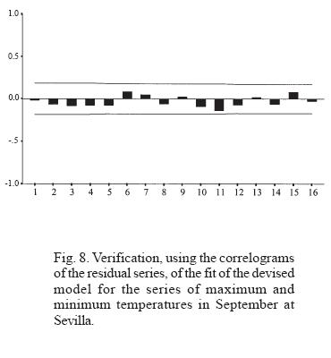
An autoregressive process of order p for the variable temperature {T_t} is represented by the equation

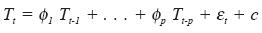
where f are the parameters whose acceptance has been previously validated. In the same way, a moving average process of order q is represented as

where {ε_t} is a white noise process, with e_t independent of the T_t-1 values, and c is a constant.

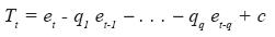
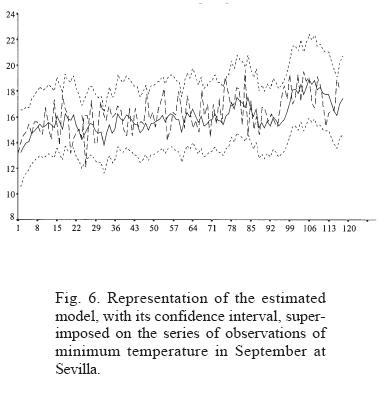
Identification of the ARIMA model that represents the organized component of each series, besides being necessary before predictions can be made, is intrinsically valuable for establishing the time organization of the set of observations and for characterizing the internal structure of each series (Figures 6 and 7). The order of the parameters (p, d, q) of the model indicates the relationships between consecutive elements of the meteorological variable, and knowing it enables comparative classifications. As a mathematical model, autoregressive moving average functions constitute a synthetic expression of the complex physical phenomenon which they represent in a simplified way.

Tables 2, 3, 4 and 5 include all the parameters calculated for the monthly and annual models for the observatories of the study. They enable us to establish the corresponding series estimated from the various models, and thereby obtain the residual series.

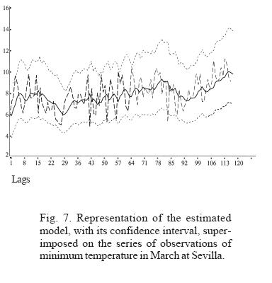
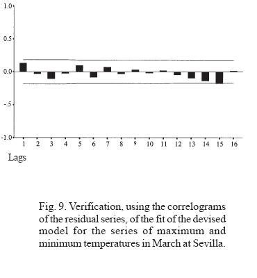
Each serial model (p, d, q) is validated from the non-correlation of its residual series. These must be random -the white noise process- with zero mean, constant variance (conditions fulfilled by the procedure applied if the series of observations is homocedastic), and non-correlated. For this, we see from the graphs of the simple autocorrelation function that all the lags are in fact within the interval of confidence. Thus, at the level of 0.95, the accepted residual correlation is significantly zero (Figs. 8 and 9).

 

5. Prediction

The first phases in devising the ARIMA model constitute an iterative process to formulate a model compatible with the structure of the data observed each month. The aim is to discover, within a level of confidence and from the knowledge of a period of effective recording, the subsequent behaviour of the series. The model devised is thus used in estimating the future values of the variables under study. The equations of the model, fitted by the elements of the series for 1< t < n, are used to progressively calculate the results of the variable t for n+1, n+2, . . . n+i.

We fixed the end of the prediction period as the year 2010 for procedural reasons and because it coincides with proposals from other bodies. Increasing the prediction period means that it is determined by the autoregressive elements, and the statistical limits of confidence are increased such that they are no longer of any practical use. Groups of experts on climate change have chosen this date for verifying control measures, and formulating different-angled hypotheses about change in climate variables.It seems advisable to coincide with this period of analysis -rather long but without loss of reliability in the estimations.

Evidently, the statistical model devised does not introduce external actions into the generative mechanism, nor does it assume actions entering from outside the system itself. However, we have to stress that the possible effects of anthropogenic activity, and its constant intensification, are assimilated by the statistical model. Climate change has been progressively incorporated throughout the period of recordings and has affected the meteorological variables under study in this research. The formulated prediction implies that the actions on the climate system will continue in the near future, similar in intensity and progression to those of the recent past.

As a result of the methodological process described above (Tables 6, 7, and 8) the monthly predictions of maximum and minimum temperatures at the observatories of Badajoz, Sevilla, and Córdoba until the year 2010, from ARIMA models, are included. We should point out that expression of the annual predictions in hundredths of °C is only of mathematical interest for observing variations between years; from the point of view of climatic significance, the precision for temperature is of tenths of a degree, as in the records of the series.

In order to compare the change obtained from preceding studies on the linear trend of the set of historical series with the future predictions from the devised models, we calculated the seasonal and annual values from the respective monthly estimations. Tables 9 and 10 present the trend of the series of historical data and the future estimations.

In the estimation of maximum temperatures, the warming in spring, common to all the observatories -and very intense at Badajoz- is striking, when, historically, they have remained stable. There is a marked divergence in thermal behavior predicted for the summers: A rise at Córdoba and fall at Sevilla, reflected in the annual warming at Córdoba against the cooling at Sevilla. The lack of statistical significance for the historical trend, and its inconstancy from one observatory to another, perhaps lead to predictions that are not concordant.

The predictions for minimum temperatures at Badajoz are similar to those at Sevilla (perhaps as a result of the relative similarity of the monthly orders of the respective p, d, q models). At Córdoba, the magnitude of the predicted decrease in winter minimum temperatures is surprising, and moderates the annual general warming. In contrast, both Sevilla and Badajoz show an even greater intensification of the rising trend for the near future, in accord with the results obtained by extrapolation of the polynomial line of the historical series.

 

6. Conclusions

Autoregressive Integrated Moving Average (ARIMA) models have been devised for the long-term monthly series of maximum and minimum temperatures from observatories in south-west Spain. Previously, it was confirmed that the first derivation and logarithmic transformation stabilized the mean and variance of the original series, and converted them into stationary series.

The orders (p, d, q) for each monthly series have been obtained. The series of minimum temperatures with one order of derivation and logarithmic transformation have been fitted to pure moving average (MA) models (38%) -above all MA(1)- to autoregressive (AR) models (58%) -mostly AR(2)- and to some mixed (ARMA) models (4%). The maximum temperatures fit principal moving average models MA( 1), with very similar monthly values for Badajoz and Sevilla, whereas at the Córdoba observatory, the predominating models are autoregressive, AR (3).

The parameters θ_p, Φ_q of the estimated functions of the monthly stochastic models have also been obtained, and subjected to validation processes to test whether the corresponding series of residuals are random. These values, and the residual variance, are given in the respective tables.

From the estimated functions for each month, predictions of change have been formulated: Those from the ARIMA models of minimum temperature suggest that the study region is in a phase of annual mean thermal increase of the order of 0.2 °C in the next decade. However, the change in maximum temperatures is not significantly defined. These estimations are in agreement with those obtained in earlier studies using other methods, but because of the better goodness-of-fit, the level of precision is much higher in this case.

 

References

Al-awadhi S. and J., Jolliffe, 1998. Times series modelling of surface presure data. Int. J. Climatol. 18, 443-455.        [ Links ]

Bravo, J. L., M. M. Nava and C. Gay, 2001. Linear and regressive stochastic models for prediction models of daily maximum ozones values at Mexico City atmosphere. Atmósfera 14, 113-123.        [ Links ]

Box, G.E.P. and G. M. Jenkins, 1970. Time Series Analysis, Forecasting and Control. Holden-Day. San Francisco.        [ Links ]

Chatfield, C., 1992. The analysis of time series. Chapman & Hall. London.        [ Links ]

Ferrand, M., 1997. Programación y análisis estadístico. MacGraw-Hill. Madrid.        [ Links ]

García-Barrón, L., 2000. Análisis de series termopluviométricas para la elaboración de modelos climáticos. Universidad de Sevilla.        [ Links ]

García-Barrón, L. and M. F. Pita, 2001. Propuesta metodológica para la determinación de inhomogeneidades relativas en las series de observaciones. El tiempo del clima. Publicaciones de la Asociación Española de Climatología, serie A Vol. 2, 87-96.        [ Links ]

García-Barrón, L., 2002. Un modèle pour l'analyse de la sécheresse dans les climats mediterranéens. Publications de 1'Association Internationale de Climatologie 14,67-73.        [ Links ]

Garrido, J. and J. A. García, 1994. Aplicación de procesos autoregresivos-media móvil para modelizar series temporales de precipitación mensual en la España peninsular. Anales de Física 89, 50-56.        [ Links ]

Grieser. J., S. Trömel and C. Schönwiese, 2002. Statistical time series decomposition into significant components and application to European temperature. Theor. Appl. Climatol. 71, 171-183.        [ Links ]

Hurrell, J. M., 1995. Decenal trends in North Atlantic Oscillation and relationship to regional temperature precipitation. Science 269, 676-679.        [ Links ]

Kendall, S. M. and J. K. Ord, 1990. Time series. Edward Arnold, London.        [ Links ]

Matyasovszky, I., 2002. A nonlinear approach to modeling climatological time series. Theor. Appl. Climatol. 69, 139-147.        [ Links ]

Martin M., L. V. Cremades and J. Santabarbara, 1999. Analysis and modelling of times series of surface wind speed and direction. Int. J. Climatol. 19, 197-209.        [ Links ]

Peña Sánchez de Rivera, D., 1995. Estadística, modelos y métodos. Alianza Universitaria, Madrid.        [ Links ]

Pita López, M. F., J. M. Camarillo and M. Aguilar, 1999. L'evolution de la variabilité pluviometrique en Andalousie (Espagne). Publications de 1'Association Internationale de Climatologie 10, 313-321.        [ Links ]

Pozo-Vázquez, D., M. J. Esteban-Parra, F. S. Rodrigo and Y. Castro-Díez, 2000. An analysis of the variability of the North Atlantic Oscillation in the time and the frecuency domains . Int. J. Climatol. 20, 1675-1692.        [ Links ]

Solange, L. and J. Pinto Peixoto, 1996. The autoregresive model of climatological times series: an aplication to the longest times series in Portugal. Int. J. Climatol. 16, 1165-1173.        [ Links ]

Uriel, Z., 1995. Análisis de series temporales. Paraninfo, Madrid.        [ Links ]

Wei, W. W., 1990. Times series. Addison-Wesley, Redwood City.        [ Links ]

Zekai S., 1998. Small sample estimation of the variance of times-averages in climatic times series. Int. J. Climatol. 18, 1725-1732.        [ Links ]