Objective analysis of daily extreme temperatures over
Indian region

 

M. MAHAKUR, S. G. NARKHEDKAR, S. K. SINHA and P. N. MAHAJAN
Indian Institute of Tropical Meteorology
Dr. Homi Bhabha Road, Pashan
Pune - 411008, India.
E-mail: mmahakur@tropmet.res.in

 

RESUMEN

Se desarrolló un esquema de análisis objetivo para estudiar las temperaturas diarias máximas y mínimas sobre la región de la India. Se utilizaron los datos diarios disponibles en el Departamento Meteorológico de la India de 1970 a 1980. Se calcularon por separado la autocorrelación y la estructura de las funciones de estos dos campos para cada mes del año. Debido a la fuerte anisotropia inducida por las características morfológicas de cierta región, se hizo un modelo de las autocorrelaciones observadas utilizando una función que no sólo considera la distancia entre dos localidades sino también sus diferencias en altitud. El esquema de análisis es la interpolación óptima, utilizando los dos tipos de funciones de correlación.

 

ABSTRACT

An objective analysis scheme to analyze daily maximum and minimum temperatures over Indian region has been developed. The daily data from 1970 to 1980 which are available with the India Meteorological Department have been used. The autocorrelation and structure functions of these two fields have been computed separately for every month of the year. Due to the strong anisotropy induced by the morphological characteristics of certain region, the observed autocorrelations have been modeled by a function which is not only a function of distance between two locations but also a function of their difference in elevation. The analysis scheme is optimum interpolation (using both types of correlation functions).

Key words: Anisotropy, maximum and minimum temperatures, optimum interpolation.

 

1.  Introduction

Essentially, there are two methods of analyzing the randomly distributed meteorological parameters. One method may be called subjective, the other objective. Among the variety of objective analysis schemes, optimum interpolation (OI) has become very popular in the last decades for the interpolation of atmospheric and oceanographic observations. The purpose of all the analysis schemes is to provide initial state data for the NWP models that are as accurate as possible. It is, however also of interest to analyse other variables, that are not used in the initial state of the model. Examples of these variables could be the temperature at the 2 metre level, precipitation, visibility and fog. In the present work optimum interpolation method (Eliassen, 1954; Gandin, 1965) is applied to analyse maximum and minimum temperatures over Indian region. Attempts have been made to highlight the importance of anisotropic effects in correlation functions due to the non-homogeneity. Cacciamani et al. (1989) have made mesoscale objective analyses of daily extreme temperatures in the Po valley of northern Italy. Their study shows strong anisotropy due to the morphological characteristics of the region.

In section 2 a brief description of OI scheme is included. Section 3 describes about the data, section 4 describes the derivations of autocorrelation functions, statistical structure functions from the historical data set and the analysis results. In section 5 conclusions have been drawn.

 

2.  Methodology

Statistical interpolation instead of optimum interpolation would be more appropriate because the autocorrelation functions, structure functions and the background fields are generally derived from the analysis of historical data series, hence what we know is a statistical estimate and not the true values. Nevertheless we will use the acronym optimum interpolation in this study. We now briefly describe the OI scheme and for detail description one can refer the classical books by Thiébaux and Pedder (1987), Daley (1991).

Let f denotes any scalar field. Subscripts i and j refer to observation points and g refers to grid point. Superscripts t, o and p refer to true, observed and background fields (predicted value) respectively. denotes the value of where bar denotes average over number of cases. In this notation, OI scheme is given by

......................................(1)

where n is the number of measuring stations and w_j are the analysis weights and depend on the autocorrelation field of the parameter to be examined. Analyzed values at the grid point are given by

...................................................(2)

where f_g^a, f_g^p represent analyzed and predicted values at the grid point g, is the spatial correlation coefficient, is normalized observational error variance, d_ij is Kronecker delta, observational error variance and is background error variance. In order to calculate w_j it is necessary to know autocorrelation field of the parameter which can be done by analyzing long time series. The observational error variance required for calculation of λ² is obtained from structure function. If and are the anomalies of true values then true structure function

.............................................................(3)

and the estimated structure function

..............................................................(4)

are related through the following relation

.....................................................(5)

becomes zero when r_ij becomes zero need not become zero at the same location. So when r_ij becomes zero, . In other words, is estimated by fitting a curve to the computed structure function, plotted against distance, r_ij and extrapolating the curve until it intersects the axis of at r_ij=0.

 

3.  Data

A historical data set of maximum and minimum daily temperatures (January to December; 1970-80) which were measured at 144 locations over Indian region were used to compute autocorrelation and structure functions. The geographical locations of the stations are shown in Figure 1. Among the original 144 stations, 134 were actually used for the optimum interpolation and remaining randomly selected 10 stations were left as references for comparison. The domain selected for this analysis is from 68°E to 98°E longitude and from 8° N to 36°N latitude cast in a 1° by 1° latitude/longitude grid. Those grid points which are in the Indian main land were considered for analyses.

 

4.  Results and discussions

4.1 Autocorrelation and structure functions

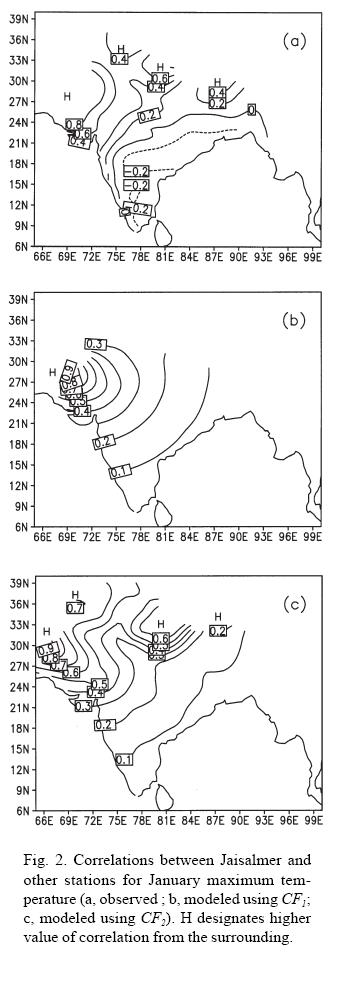
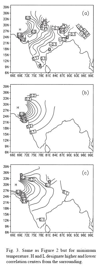
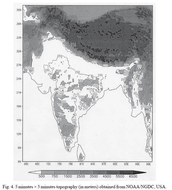
In order to solve the equation (1) we must have the knowledge of the autocorrelations (C_ij and C_gi) and structure functions. Based on 11 years (1970-1980) data, covariances and structure functions for each month (January to December) and for both maximum and minimum temperature were computed. These computed covariances were normalized by dividing them with the corrected variances . Normally in OI scheme autocorrelation functions are assumed to be homogeneous and isotropic and the analytical functions which are used to model the observed autocorrelations are assumed to be functions of only distance between two locations. Thiébaux (1976), Seaman and Gauntlett (1980) have shown that these assumptions are not valid in the case of surface parameters. Figures 2a and 3a show that the spatial observed correlation patterns for maximum and minimum temperatures between Jaisalmer station (26.90°N, 70.92°E) and the remaining stations during the month of January. It can be observed that the correlation decreases with increasing distance from the Jaisalmer station for both maximum and minimum temperatures. From the observed patterns of the correlation it can be seen that the spatial structure of the correlations are not isotropic. Panels (b) and (c) of Figures 2 and 3 will be discussed later. Figure 4 shows the 5 minutes x 5 minutes topography (in meters) obtained from NOAA/NGDC (National Geophysical Data Center), USA. Elevations greater than 500 meters have been shaded. Peak elevation around 7500 meter can be observed over the Tibetan Plateau of Himalayas in the extreme north. Also another peak around 1500 meter can be observed over the western ghats along the west coast of India and Deccan Plateau. Also surface elevations around this peak can be seen on the central parts of India (such as Aravalli range, Chota Nagpur, Vindhyas range) and eastern ghats along east coast. These complex terrains up to some extent are responsible for the anisotropic pattern of observed correlations, which is evident from following discussion. However, station observations over this elevated terrain are sparse (Fig. 1).

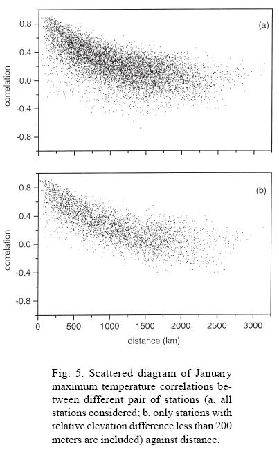
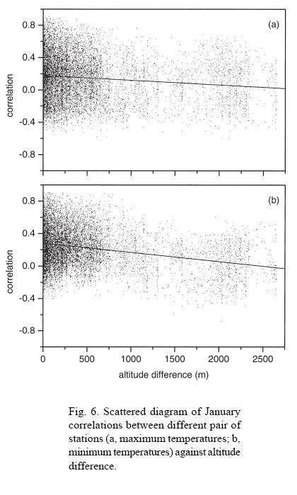
Scatter plots of correlations of maximum temperatures versus station separations for the month of January are shown in Figure 5(a). This diagram also shows the general tendency of decreasing correlations with increasing distance as stated earlier. This is irrespective of their elevation differences. From this diagram it can be seen that observed correlations become negative at small station separation as small as around 108 km. Similar plot is made in panel (b) of Figure 5 considering only those pairs of stations whose absolute elevation differences are less than 200 meter. It can be seen from Figure 5(b) that correlations are becoming negative when station separations are around 465 km or more. This shows that closest stations are not always most correlated due to the effect of topography. Also it can be observed from Figure 5(b) that minimum correlation observed is -0.3 when stations with elevation difference more than 200 meters are excluded. On the other hand, minimum correlation of -0.7 is observed when all the pairs of stations are considered (Fig.5a). It is evident from Figure 5(b) that correlations are less scattered when elevation difference less than 200 meters is considered as compared to Figure 5(a). This shows the role of station elevation in making correlation anisotropic to some extent. Figure 6 shows the scatter plot of correlation versus absolute station elevation difference between pair of stations during the month of January. Panel (a) is for maximum temperature and panel (b) for minimum temperature. Although the correlations are highly scattered the clear decreasing trend in correlations with increasing altitude difference can be noted from the best-fit line for maximum and minimum temperatures. This decreasing correlation with increasing elevation difference was also observed in both maximum and minimum temperatures for all other months (figures not shown).

Thus on the basis of the above discussions it can be inferred that correlation is not only a function of distance but also of absolute altitude difference and the later account for the anisotropy of the correlation up to some extent. Figure 7(a) shows isolines of correlations for January maximum temperature measured at Nagpur station (21.10°N, 79.05°E) and Figure 7(b) shows isolines of correlation for April maximum temperature measured at the Jaisalmer station. Looking at the Figure 2a and Figures 7a, b it can easily be stated that correlation not only depends on distance but also is dependent on other morphological features (such as elevation) and season. In addition correlation patterns for maximum and minimum temperatures are different (Figs. 2a and 3a). Thus the correlation functions for maximum and minimum temperatures have to be modeled separately and for each months of the year.

The observed correlations are modeled by two different exponential functions:

...................................................(6)

......................(7)

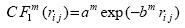
where 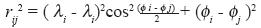is the distance between two stations i and j, λ and Φ are longitude and latitude of the stations, m =1,2, ...,12 is the month of the year, a, b, c are the coefficients, and is the absolute value of the elevation difference between stations i and j CF₁ is a isotropic function which do not include elevation difference during modeling of observed correlations whereas CF₂ takes into account elevation difference along with the station separations during modeling. Figure 8 shows the variation of the constants a, b^-1 and c^-1 from month to month, panel (a) for maximum temperature and panel (b) for minimum temperature for CF2. The observed correlations for the month of January maximum temperature (Fig. 2a) have been modeled with CF₁ (Fig. 2b) and CF₂ (Fig. 2c). Now comparing the panel of three diagrams Figures 2a, 2b and 2c, we found that observed structure of correlations is well captured by CF2 but CF₁ failed to capture the observed structure. It can be noted that higher values of correlations in the north and northeast India which are seen in Figure 2(a) are completely absent in CF₁ (Fig. 2b) but CF₂ (Fig. 2c) is able to retain these observed structures. Similarly in the case of minimum temperature (Fig. 3), the observed correlations (Fig. 3a) of January have been modeled with CF1 (Fig. 3b) and CF2 (Fig. 3c). In this case, also it is found that CF₂ is slightly better than the CF₁. Similar to Figures 2 and 3, Figures 9 and 10 show the observed and modeled correlations with respect to Jaisalmer station during July month for maximum and minimum temperatures respectively. Observed negative correlations are shaded in panels (a) of Figures 9 and 10. It can be seen that correlations modeled using CF₂ are better than modeled by CF₁ specifically for minimum temperature. From Figures 9a and 10a, it can be seen that the observed correlation becomes negative after shorter distance as compared to January month (Figs. 2a and 3a) showing correlations are local during July month as compared to January month. This is also corroborated by b^-1 values from the middle panels of Figures 8a and 8b.

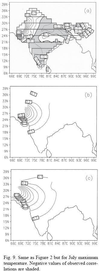
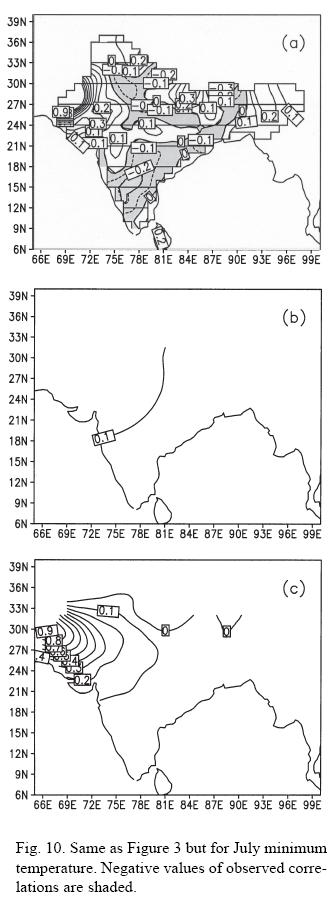
Figure 11 shows the plot of variance for every month of the year for both maximum and minimum temperatures. It is noticed that variance for the maximum temperature is less during winter and increases slowly and is maximum (highest) in June, 11°C². The variance of minimum temperature is generally less than the maximum temperature from March to September with rapid increase from October to February. An interesting pattern is the presence of peaks and troughs in the variance of maximum temperature centered in March, April and June, whereas variance of minimum temperature has troughs in August, September and peak in November. Thus for both maximum and minimum temperatures two types of climatological regime are evident, i.e. a summer type during which variances of maximum temperature are higher than the minimum temperature whereas during winter it is other way. In Figure 12 the random error for maximum and minimum temperature for every month of the year are plotted. It is observed that random errors for minimum temperature are generally higher than the maximum temperature throughout the year (except July).

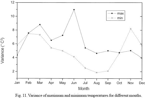
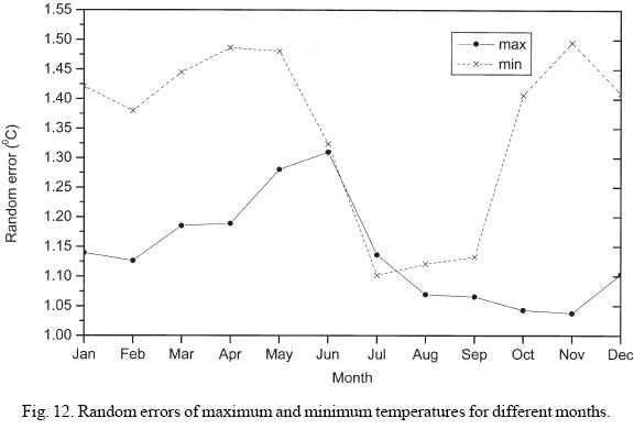
Figure 8 shows the value of the coefficients a, b^-1 and c^-1 of the function CF₂ for different months of the year. Panel (a) is for the maximum temperature and (b) for the minimum temperature. From this diagram, it can be noted that vertical length scale c^-1 is two orders of magnitude less than the horizontal length scale b^-1 for both maximum and minimum temperatures. This shows the strong effect of elevation difference than the station separation between two stations for both maximum and minimum temperatures. Findings of Cacciamani et al. (1989) are similar to our findings in the case of minimum temperature, whereas in the case of maximum temperature they are (b^-1 and c^-1) of the same order particularly during the summer months (June-August). It was observed that the vertical length scale c^-1 for the maximum temperature is large during rainy season (June-August), whereas c^-1 is small for winter and summer months. Generally c^-1 increases from January to June and then decreases. Thus from the above observations it can be inferred that the effect of elevation difference is more during winter and summer months. The value of c^-1 for minimum temperature is less than that of maximum temperature. Hence for the case of minimum temperature the influence of elevation difference is much more as compared to maximum temperature and remains almost same throughout the year except during July to October when the effect is slightly more. The horizontal length scale is higher during the colder months and in March for both maximum and minimum temperatures. Comparing the horizontal and vertical scale length (maximum temperature) it is found that station separation is more dominant during rainy season than in other months of the year. It is other way for the elevation difference. For the case of minimum temperature the elevation difference and station separation both are dominating during the rainy season than the other months. The bottom diagram of panels (a) and (b) of Figure 8 shows the zero intercept a of CF₂ for all the months of the year for maximum and minimum temperatures when both the horizontal distance and the elevation difference are zero.

4.2 Analysis of results

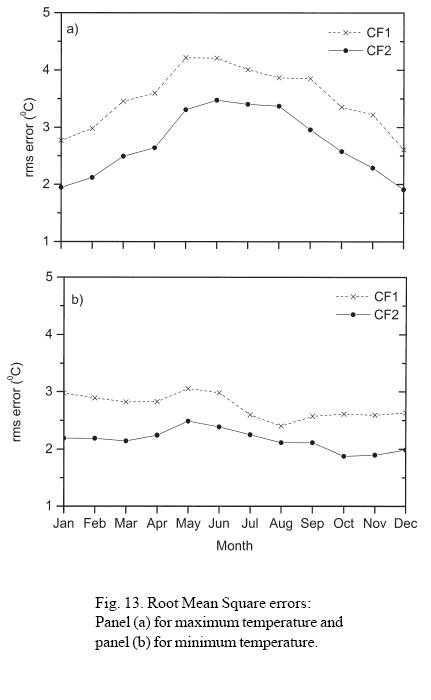
First guess (f_g^p) plays an important role on the performance of any objective analysis scheme. It may be climatology, persistence or an output from a numerical weather prediction model. Since we do not have forecast value of daily maximum and minimum temperature from numerical model and as climatology is independent of the characteristics of the model, we have decided to use climatology as first guess. As mentioned earlier daily objective analysis over Indian region for maximum and minimum temperature for the period 1970 to 1980 were carried out. It is necessary that the analyses produce realistic field and a better way to validate this is to compare the analysis against independent data not used in the analysis. The cross validation approach to assess the analysis has been used in this study. Out of 144 stations, 10 stations (indicated by '+' in Fig. 1) were excluded to compute independently root mean square (rms) error between observed and analyzed values. In Figure 13 rms errors for maximum (panel a) and minimum (panel b) temperatures are shown. It is observed that rms errors of analysis using CF₂ function are lower than the analyses using CF₁ for both maximum and minimum temperatures. It can be observed that in the case of maximum temperature (Fig. 13a) the interpolation using CF₁ as well as CF₂ performs differently in different seasons. The performance is better during the winter season than that of the summer and rainy season, but it is not the case for minimum temperature (Fig. 13b). It is to be noted that error with CF₂ for maximum temperature is lower than minimum during winter (December, January and February) and higher during summer. This is because the former is more local than the later during the warm season and vice versa during the cold season. The difference in error between CF₂ and CF₁ for both maximum and minimum temperatures is smallest in July and August. The observed correlations were also modeled using squared exponential function for both isotropic (CF₃) and anisotropic case (CF₄):

.................................................(8)

...................(9)

The values of A, B^-1, C^-1 gave similar results as of Figure 8. Again, the rms errors obtained for both maximum and minimum temperatures using CF₃ and CF₄ are less than that of CF₁ and CF₂ during all the months of the year (figure not shown). In addition, error due to CF₄ is less than that of CF₃. This has clearly brought about the importance of modeling the observed correlation with a function which is not only a function of horizontal station separation but also is a function of their elevation difference.

 

5. Conclusions

An optimum interpolation scheme has been developed to analyze surface maximum and minimum temperatures over Indian region. Autocorrelation and structure functions, which are necessary for the objective analysis, have been computed based on 11 years of data. While performing objective analysis, 10 stations are excluded to compute the rms errors. The following conclusions are drawn.

Due to anisotropy, the autocorrelation functions have been modeled with a regression equation, which is not only a function of station separation but also the absolute value of elevation difference between stations. Thus, the main idea of the present work is the usage of the elevation difference between stations to estimate the analysis weights. The coefficients a, b^-1 and c^-1 of CF₂ and A, B^-1 C^-1 of CF₄ depend strongly on the season. So far the measure of rms errors are concerned, the analysis obtained by modified function CF₂ and CF₄ is comparatively better than CF₁ and CF₃ for both maximum and minimum temperatures. In the case of maximum temperature, the interpolation is better during winter than the summer and rainy season.

 

Acknowledgements

The authors would like to thank Dr. G.B. Pant, Director, Indian Institute of Tropical Meteorology, Pune for his constant encouragement and Dr. S.S. Singh, Head, F.R.D. for his interest in this study. Thanks are also due to India Meteorological Department for the extreme temperature data and NOAA/NGDC, USA for providing the 5-minute terrain data and the GeoVu software.

 

References

Cacciamani, C., T. Paccagnella, S. Nanni and S. Tibaldi, 1989. Objective mesoscale analysis of daily extreme temperatures in the Po valley of Northern Italy. Tellus 41 A, 308-318.        [ Links ]

Daley, R., 1991. Atmospheric data analysis. Cambridge University Press, Cambridge.        [ Links ]

Eliassen, A., 1954. Provisional report on calculation of spatial co variance and autocorrelation of the pressure field. Institute of Weather and Climate Research, Academy of Sciences, Oslo, Report No. 5.        [ Links ]

Gandin, L. S., 1965. Objective analysis of meteorological fields. Israel Program for Scientific Translation, Jerusalem.        [ Links ]

Seaman, R. S. and F. S. Gountlett, 1980. Directional dependence of zonal and meridional wind correlation coefficients. Aust. Met. Mag. 28, 217-218.        [ Links ]

Thiébaux, H. J., 1976. Anisotropic correlation functions for objective analysis. Mon. Wea. Rev. 104, 994-1002.        [ Links ]

Thiébaux, H. J. and M. A. Pedder, 1987. Spatial objective analysis. Academic Press, London.        [ Links ]