The Lorenz chaotic systems as nonlinear oscillators with memory

 

S. Panchev
Solar Terrestrial Influences Laboratory, Bulgarian Academy of Sciences, 1113 Sofia,
Bulgaria and Faculty of Physics, Sofia University, 1164 Sofia, Bulgaria
e-mail: spanchev@phys.uni-sofia.bg

T. Spassova
National Institute of Meteorology and Hydrology, Bulgarian Academy of Sciences,
1784 Sofia, Bulgaria
e-mail: tatiana.spassova@meteo.bg

 

RESUMEN

Los sistemas no lineares dinámicos (sistemas de ecuaciones diferenciales ordinarias de 1er orden) capaces de generar caos son no integrables analíticamente. A pesar de esto, se pueden utilizar herramientas analíticas para extraer información útil de ellas. En este trabajo el sistema original de Lorenz y sus modificaciones se reducen a ecuaciones oscilatorias únicas de tipo integral-diferencial con argumento retrasado. Esto lleva a la aparición de un término "endógeno" que se interpreta como memoria para el pasado. Por otra parte, las ecuaciones son válidas más allá del instante inicial (teóricamente en t ->∞), cuando el sistema evoluciona hacia su conjunto atractor. Esto corresponde a las soluciones numéricas cuando una parte inicial adecuada del iterato generalmente se descarta para eliminar a los transitorios. Además la forma de las ecuaciones permite su tratamiento estadístico.

 

ABSTRACT

Nonlinear dynamical systems (systems of 1st order ordinary differential equations) capable of generating chaos are analytically nonintegrable. Despite of this fact, analytical tools can be used to extract useful information. In this paper the original Lorenz system and its modifications are reduced to single oscillatory type integral-differential equations with delayed argument. This yields to appearance of an "endogenous" term interpreted as memory for the past. Moreover, the equations are valid far from the initial instant (theoretically at t->∞), when the system eventually evolves on its attractor set. This corresponds to the numerical solutions when an appropriate initial part of the iterates is usually discarded to eliminate the transients. Besides, the form of the equations allows statistical treatment.

Key words: Chaotic systems, memory function, Duffing oscillator.

 

1. Introduction

In principle, any system of n first order nonlinear ordinary differential equations (ODE) can be transformed into lower number higher order, or to integral-differential equations by means of consistent elimination of dependent variables. In doing so in this paper, we will need some preliminary mathematical derivations:

Let

...........................................(1.1)

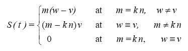
be a differential equation for u(t) with given functions v(t), w(t), initial values u₀, v₀ and parameters k, l, m, n. Alternatively,

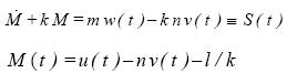............................................(1.1a)

The general solution of (1.1a) is

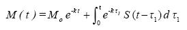
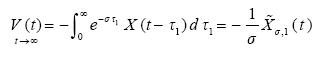
Hence, the long time (t->∞) behaviour of the solution will be governed by

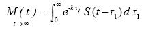........................................................(1.2)

or

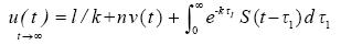....................................(1.2a)

According to (1.1 a)

.......................(1.3)

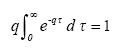
Therefore, the current time value u(t) is determined not only by S(t), but by S(t - ) as well, the latter being exponentially suppressed. It is reasonable to interpret the integral term in (1.2) as a kind of memory, remaining after the transient has passed (t ->∞). To characterize this effect, following Festa et al. (2002), we introduce the memory function

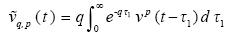.................................................(1.4)

with p=1 (linear memory) or p=2 (quadratic memory). For example, if , v(t)=sint then

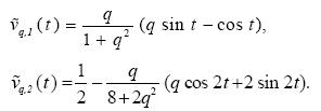
Obviously 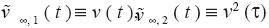, and

..........................................................................(1.5)

If v(t) is a random function (Panchev, 1971), will be a random one too and can be treated statistically (see section 4 below).

Equations of the type (1.1) and its solution (1.2) occur in the theory of motion of Stokes' particles in turbulent flow and of linear measurement devices with inertia, e. g. some meteorological instruments (Panchev, 1971, ch. 8).

Here we apply the previous results to the original Lorenz low order system of ODE (section 2) and to its modifications (section 3). In section 4 we show how the obtained solutions of the type (1.2) can be treated statistically. Some conclusions are formulated in section 5.

 

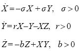
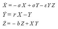
2. The original Lorenz (1963) system

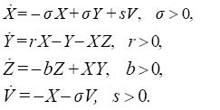
The system is a 3-dimensional, 3-parametric one

................................................................(2.1)

For r > 1 it has two nonzero fixed points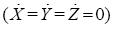

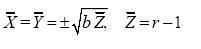..........................................................(2.2)

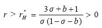
At σ > b+1 and

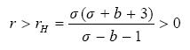.......................................................(2.3)

the system exhibits chaotic behaviour. Otherwise chaotic regime is impossible. A combination between X- and Z-equations of (2.1) yields

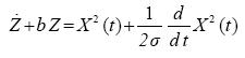.....................................................(2.4)

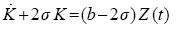
It can be rewritten as

...........................................................(2.5)

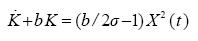
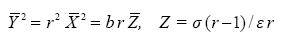
where

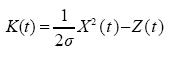................................................................(2.6)

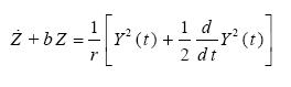
Alternatively from (2.1) and (2.6) we derive

...............................................................(2.7)

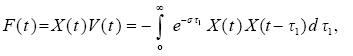
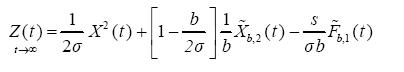
Equations (2.4) - (2.7) are of the type (1.1), so that at t->∞ the solution (1.2) can be used directly. Thus,

.............................................................(2.8)

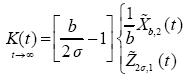
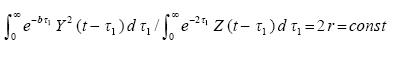
respectively. Hence, it follows that

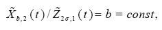...................................................(2.9)

which is the same as

...............(2.9a)

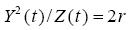
If b=2σ, i. e. r_H in (2.3) does not exist, then K(t)=0 and (2.8) yields

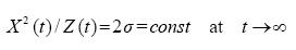............................................(2.10)

It is worthwhile to compare (2.9) - (2.10) with (2.2) .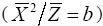

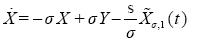
So far, the second equation of the system (2.1) was not used. Eliminating Y(t) and Z(t) one obtains

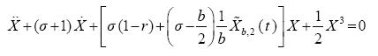.............(2.11)

which is the forced Duffing oscillator. Through (2.9) can be introduced instead of . Equation (2.11) governs the final behaviour of the system (2.1) at t->∞, when it lies and permanently evolves on its attractor set, eventually oscillating around the two unstable fixed points (2.2). This state is self-sustained by the memory term in (2.11). As it follows from (2.8), the memory is carried either by X- or by Z -variables in (2.1), but with different memory decay time (in the Lorenz time units) - 1/b and 1/2σ. Besides, the memory term vanishes if b=2σ. However, this is not the case with the traditional Lorenz values b=8/3, σ=10, r=28, when (2.1) and consequently (2.11) behaves chaotically.

Being in force at t->∞, the invariant ratio (2.9) can be used as a criterion for numerical evaluation of the practical duration of the initial transient. Moreover, how fruitful can be the representation of (2.1) in the oscillatory form (2.11) was recently shown in Festa et al. (2002) .

 

3. Quasi-Lorenz systems

We call quasi-Lorenz systems those that are "derivatives" (modifications) of the original one (2.1). Such a system was studied in Panchev (2001), and Panchev and Spassova (1999).

............................................................(3.1)

where σ, ε, r, b > 0. Unlike (2.1), the first equation is nonlinear while the second one is linear. At r >1 there exist two nonzero fixed points determined by

.........................................(3.2)

Moreover, at σ + b < 1 and

..........................................................(3.3)

the qualitative behaviour of (3.1) follows that of (2.1) under the conditions (2.3).

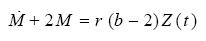
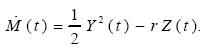
The last two equations of (3.1) yield

.............................................(3.4)

It can be written in two alternative forms:

...........................................................(3.5)

and

.........................................................(3.5a)

where

........................................................(3.6)

Using again (1.2) we obtain

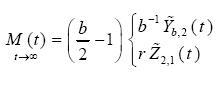.....................................................(3.7)

Hence

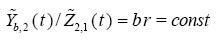.......................................................(3.8)

which is the same as

..................(3.8a)

These expressions correspond to (2.9), (2.9a). Unlike the latter, the ratios (3.8) depend explicitly on r.

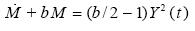
Eliminating X(t) and Y(t) in the first equation (3.1) by means of the second one and (3.6), (3.7) one obtains again a Duffing type self-forced oscillator, corresponding to (2.11):

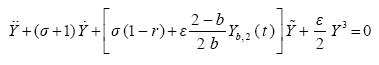......................(3.9)

As it is seen, the memory is carried either by Y- or by Z -variables with decay time 1/b and 1/2, while in (2.8) we had X and Z with 1/b and 1/2σ t decay time. Moreover, it follows from (3.7) and (3.9) that at b=2 the memory term vanishes and (3.9) degenerates into a regular Duffing oscillator. In this particular case (3.7) and (3.6) yield

.......................................................................(3.10)

corresponding to (2.10). As rigorous results from the initial systems (2.1) and (3.1) at t->∞, the invariant ratios (2.9), (3.8) and (2.10), (3.10) can be checked numerically, integrating (2.1) and (3.1).

Many other systems can be classified as quasi-Lorenz ones. We shall consider two more examples only. The first one is the four dimensional system of meteorological origin, derived in Stenflo (1996)

.................................................(3.11)

Obviously the original Lorenz system (2.1) is embedded (built) in (3.11). However, the meaning of the parameters is different from the previous ones (Stenflo, 1996).

The new equation in (3.11) implies that

.................................(3.12)

Therefore, (3.11) is equivalent to the system (2.1) with the first equation replaced by

..........................................................(3.13)

Consequently, a new term appears on the right-hand side of equation (2.4), where

...........................(3.14)

Hence, we derive the extended version of the equation (2.8)

.................(3.15)

where

.....(3.16)

Obviously, is a more complicated quadratic type memory (secondary, or mixed one).

The second example is the generalized Lorenz system in the complex domain (Fowler et al., 1983)

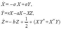...................................................(3.17)

where X(t), Y(t), a, r are complex functions and parameters, Z(t) is a real function, σ, b are real parameters and the asterisk (*) denote complex conjugate. Thus, in real quantities (3.17) is a five-dimensional dynamical system. It occurs in the theory of nonlinear baroclinic instability in the atmosphere, a problem of great meteorological significance, and also in the laser physics (Rauh et al., 1996).

Formally, (3.17) differs from (2.1) by the Z-equation. However, the latter is easy transformed into a form identical to (2.4)

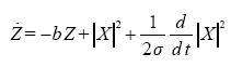........................................................(3.18)

where . Therefore, all equations (2.5) - (2.10) remain in force if X(t) is replaced by . The equation (2.11) now takes the form

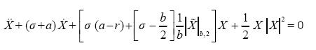.......(3.19)

It is a nonautonomous complex Duffing type equation. In the real domain it is equivalent to two coupled equations of the same type.

 

4. An example of statistical treatment

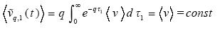
Let v(t) be a random (chaotic) function. Then the memory function is a random (chaotic) one too. In addition we assume that v(t) is a statistically stationary function (Panchev, 1971), i.e.

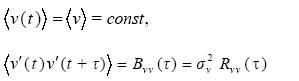......................................(4.1)

where 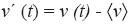is the deviation from the mean value . Obviously 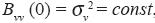, is the dispersion of v'. Under these assumptions it follows that

and

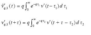
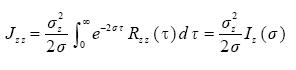
Then, for the memory autocorrelation function we obtain

.....(4.2)

after one integration has been performed (Panchev, 1971). Hence

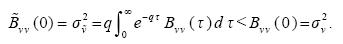.............................(4.3)

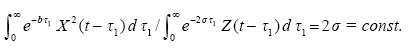
We now apply these results to the Lorenz system (2.1). As an example we take the second solution (2.8)

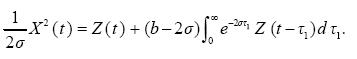...........................(4.4)

valid at t->∞. Zou et al. (1985) showed that the motion on the strange attractor is ergodic. It is reasonable to think that it is also stationary in the above sense (4.1). Thus, we can average (4.4). The result is (cf. (2.2), (2.9))

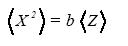........................................................................(4.5)

Subtracting (4.5) from (4.4), squaring and averaging, we obtain

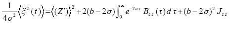
where ,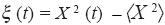

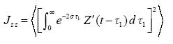
However, the squared integral equals to a double one

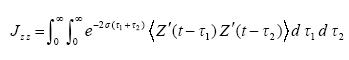
where 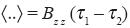is the autocorrelation function of the Z -variable. Finally (see also (4.3))

so that

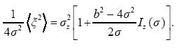................................................(4.6)

In a similar way other statistical characteristics can be computed.

 

5. Conclusion

Normally high order ordinary differential equations are transformed to dynamical systems (systems of 1st order equations), suitable for further analytical treatment and numerical solution. Here we followed the opposite procedure. Owing to the appropriate structure (1.1) of the equations in the original Lorenz low-order system (2.1) and its modifications (3.1), (3.11) and (3.17), single oscillatory type equations with forcing endogenous "memory" terms are derived, valid a t->∞. In this connection linear and quadratic memories were defined by (1.4) and (3.16). For particular relationships among the systems' parameters (b=2σ for (3.1) and b=2 for (3.11)), the memory terms in (2.11) and (3.9) vanish. The latter result is new, while the former one is already known. In both cases, the results are autonomous Duffing type equations and invariant ratios (2.10) and (3.10). Moreover, other new invariant ratios (2.9) and (3.8) are rigorously derived from (2.1) and (3.1). Section 4 demonstrates the possibilities of the statistical approach in case of final (t->∞) chaotic behaviour. The results of the previous sections may prove to be useful for various applications of the Lorenz and Lorenz-like systems, including meteorological ones.

The systems considered in sections 2 and 3 are not the only ones that can be reduced to oscillators with memory. We have collected other examples of dynamical systems (mainly 3-dimensional) that can also be transformed and treated by means of the same tools, including statistical ones.

 

References

Festa R., A. Mazzino and D. Vincenzi, 2002. Lorenz-like systems and classical dynamical equations with memory forcing: An alternative point of view for singling out the origin of chaos, Phys. Rev. E65, 046205.        [ Links ]

Fowler A. C., J. D.Gibbon and M. J. McGuiness, 1983. The real and complex Lorenz equations and their relevance to physical systems. Physica 7D, 126-134.        [ Links ]

Lorenz E. N., 1963. Deterministic nonperiodic flow. J. Atmos. Sci., 20, 130-141.        [ Links ]

Panchev S., 1971. Random functions and turbulence. Pergamom Press. Oxford, 444 p.        [ Links ]

Panchev S., 2001. Theory of chaos (2nd ed. in Bulgarian), Bull. Acad. Press. 450 p.        [ Links ]

Panchev S. and T. Spassova, 1999. The Lorenz chaotic system with modified X-, Y-equations, Bull. Cal. Math. Soc., 91, 17-28.        [ Links ]

Rauh A., L. Hannibal and N. B. Abraham, 1996. Global stability properties of the complex Lorenz model. Physica D99, 45-58.        [ Links ]

Stenflo L., 1996. Generalized Lorenz equations for acoustic-gravity waves in the atmosphere. Physica Scripta, 53, 83.        [ Links ]

Zou Chengzhi, Zhou Xiuji, and Yang Peicai, 1985. The statistical structure of Lorenz strange attractor. Adv. Atmos. Sci., 2, 215-224.        [ Links ]